Jack Mackerel Assessment SCW16
SPRFMO
South Pacific Regional Fisheries Management Organisation
Jack Mackerel Working Group
Jack Mackerel Assessment SCW16
This focused report summarizes the completed SCW16 model outputs for the SC13 baseline (0.00), the previous final bridge model (0.12), and the proposed final model (0.14). Model 0.14 starts from the acoustic-drop configuration (1.03) and adds a 2018 Peruvian CPUE catchability break; it is treated here as the proposed final model pending review. The report also includes the 0.13 catchability sensitivity, the data sensitivities completed so far (1.01-1.04), and the additional SC13 downweighting sensitivity (SC13_1.15). Two additional diagnostic trials (1.05 and 1.06) are shown separately from the data sensitivities under “Other trials.” Retrospective diagnostics are included for the proposed final 0.14 configuration under both stock-structure hypotheses; ADNUTS MCMC diagnostics were not rerun after the latest two-stock control-file updates and are omitted from this version.
1 Model Set
| Model | Role | Description |
|---|---|---|
| 0.00 | SC13 baseline | Baseline SC13 framing for the single-stock and two-stock hypotheses. |
| 0.12 | Previous final bridge model | Previous final bridging configuration; as 0.11 but with the DEPM abundance-index series removed. |
| 0.13 | Catchability sensitivity | As 0.12 but adds a 2018 catchability break for the Peruvian CPUE index. |
| 0.14 | Proposed final model | Proposed final configuration; as 1.03 but adds the 2018 catchability break for the Peruvian CPUE index. |
| 1.01 | Data sensitivity | As 0.12 but replaces `Chile_CPUE` with the 0.00 Chilean CPUE series. |
| 1.02 | Data sensitivity | As 0.12 but replaces `Peru_CPUE` with the 0.00 Peruvian CPUE series. |
| 1.03 | Data sensitivity | As 0.12 but drops `Peru_Acoust_S1` and `Peru_Acoust_S2`. |
| 1.04 | Data sensitivity | As 1.03 but adds the old 0.00 `Peru_Acoustic` index, with selectivity tied to the FarNorth fishery. |
| 1.05 | Other trial | As 0.12 but replaces `Peru_CPUE` with a noisy (CV = 60%) nominal CPUE series for 1990-2025. |
| 1.06 | Other trial | As 1.05 but removes `Peru_Acoust_S1` and `Peru_Acoust_S2`. |
| SC13_1.15 | SC13 sensitivity | Additional SC13 run that fully downweights the Acoustic N and Peruvian CPUE index series across all years. |
You’ll need to be in the jjm/assessment directory in order for the code here to run.
2 Updated Data
2.1 Datasets
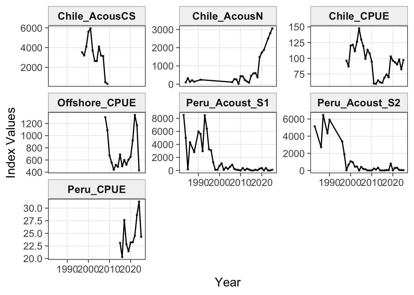
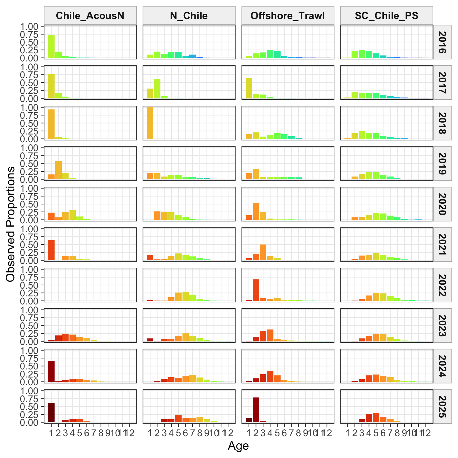
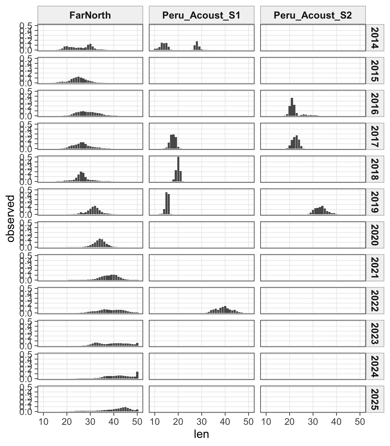
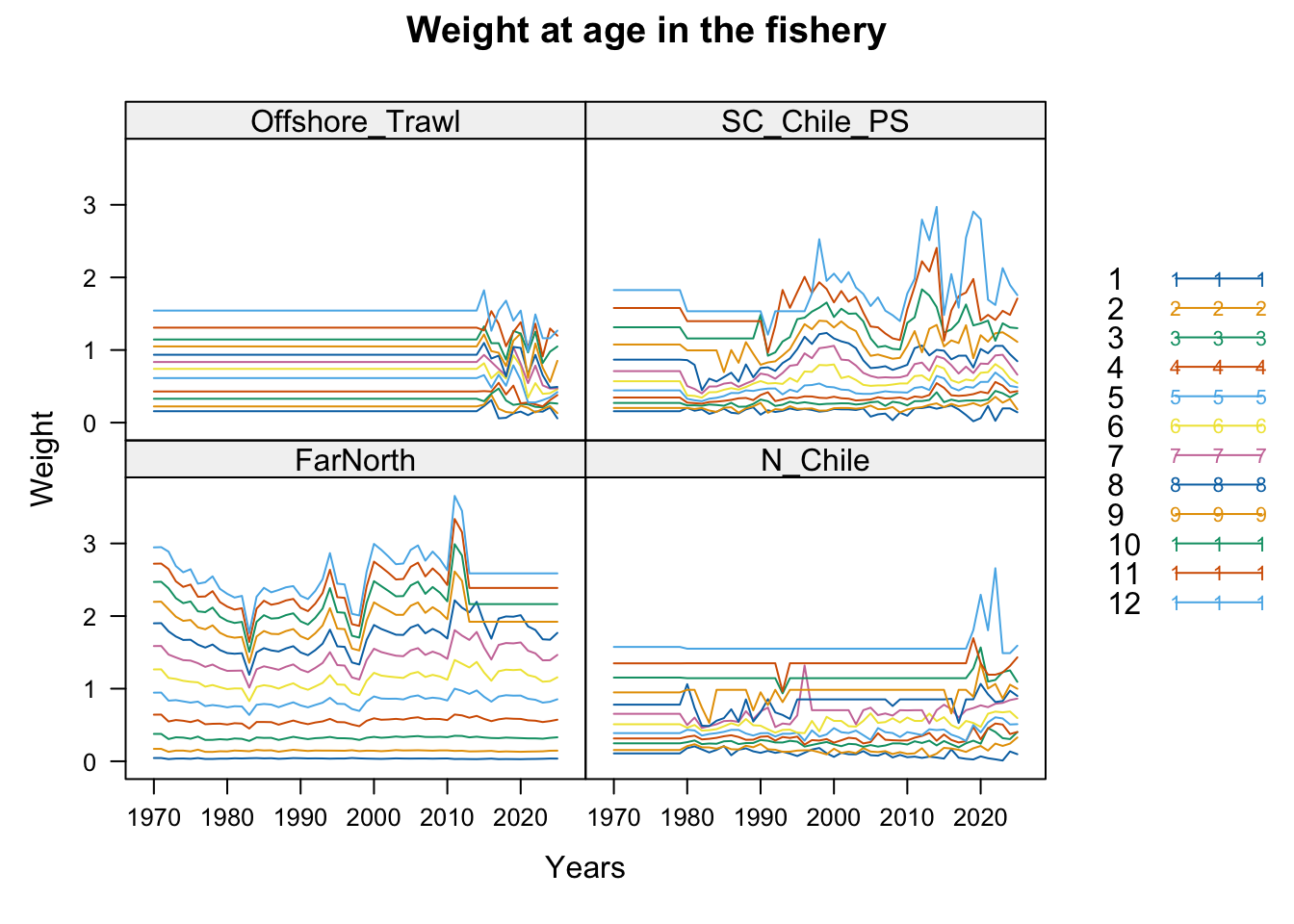
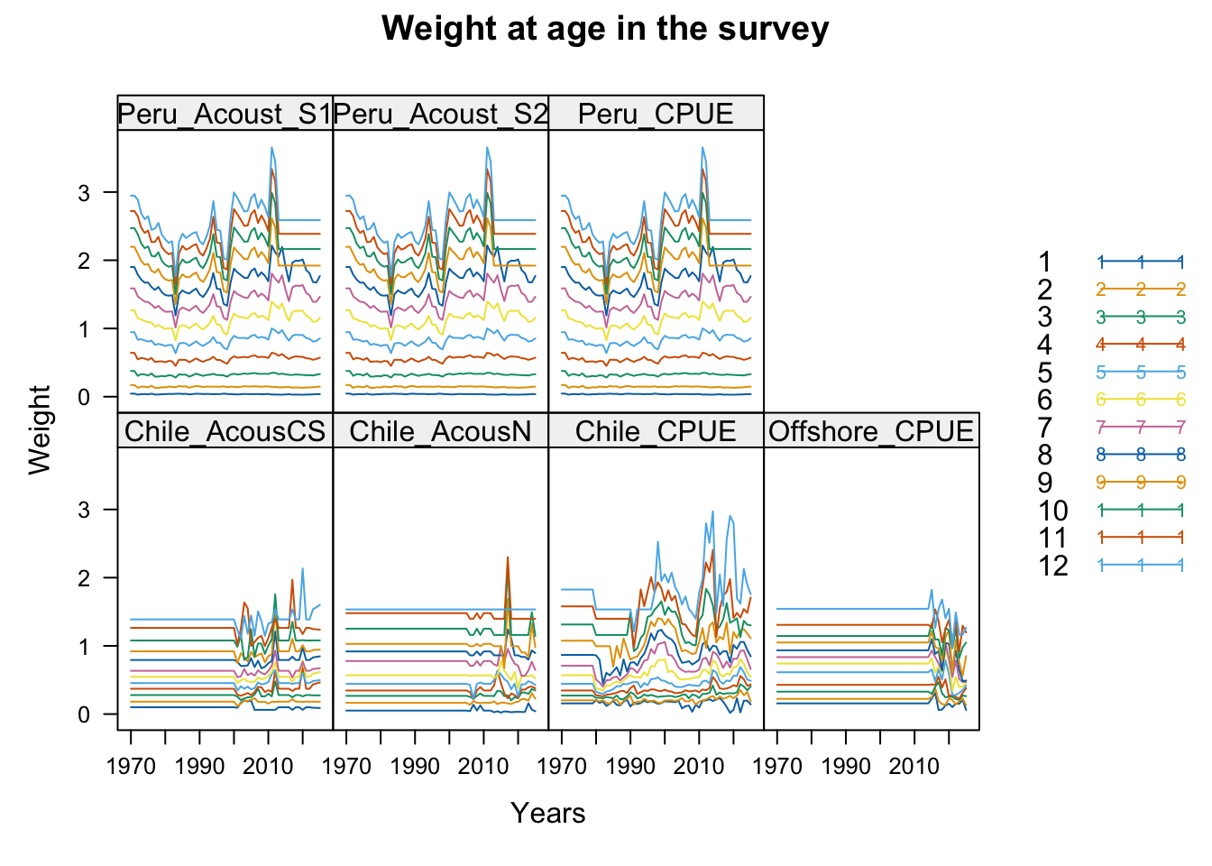
3 Fit Summaries
The fit summaries are useful for checking convergence and for comparing runs that share the same data and likelihood structure. Several rows in this table intentionally change the data configuration, so negative log-likelihood values should not be interpreted as a strict ranking across all models.
| Hypothesis | Model | Run | N parameters | NLL | Max gradient |
|---|---|---|---|---|---|
| h1 | 0.00 | h1_0.00 | 1865 | 1323.818 | 0.0002112 |
| h1 | 0.12 | h1_0.12 | 1871 | 3820.555 | 0.0003189 |
| h1 | 0.14 | h1_0.14 | 1844 | 1301.560 | 0.0003153 |
| h1 | 0.13 | h1_0.13 | 1872 | 3768.890 | 0.0002346 |
| h1 | 1.01 | h1_1.01 | 1871 | 3811.122 | 0.0002282 |
| h1 | 1.02 | h1_1.02 | 1871 | 3831.319 | 0.0002985 |
| h1 | 1.03 | h1_1.03 | 1843 | 1306.689 | 0.0002805 |
| h1 | 1.04 | h1_1.04 | 1844 | 1354.092 | 0.0003000 |
| h1 | SC13_1.15 | h1_1.15 | 1865 | 1166.248 | 0.0002013 |
| h2 | 0.00 | h2_0.00 | 1648 | 1249.606 | 0.0002636 |
| h2 | 0.12 | h2_0.12 | 1962 | 2641.727 | 0.0001820 |
| h2 | 0.14 | h2_0.14 | 1935 | 1184.311 | 0.0003320 |
| h2 | 0.13 | h2_0.13 | 1963 | 2610.178 | 0.0002511 |
| h2 | 1.01 | h2_1.01 | 1932 | 2699.890 | 0.0003842 |
| h2 | 1.02 | h2_1.02 | 1932 | 2692.811 | 0.0002865 |
| h2 | 1.03 | h2_1.03 | 1904 | 1275.404 | 0.0004646 |
| h2 | 1.04 | h2_1.04 | 1905 | 1311.022 | 0.0002846 |
| h2 | SC13_1.15 | h2_1.15 | 1648 | 1049.019 | 0.0002749 |
4 Terminal-Year Metrics
| Hypothesis | Model | Stock | Year | SSB | Total biomass | Recruitment | Max total F at age |
|---|---|---|---|---|---|---|---|
| h1 | 0.00 | Stock_1 | 2025 | 15183 | 21807 | 17018 | 0.589 |
| h1 | 0.12 | Stock_1 | 2025 | 3211 | 6342 | 10667 | 2.462 |
| h1 | 0.14 | Stock_1 | 2025 | 5773 | 9679 | 12358 | 2.162 |
| h1 | 0.13 | Stock_1 | 2025 | 4118 | 7541 | 11115 | 2.601 |
| h1 | 1.01 | Stock_1 | 2025 | 3342 | 6471 | 10365 | 1.064 |
| h1 | 1.02 | Stock_1 | 2025 | 5998 | 9922 | 11610 | 3.061 |
| h1 | 1.03 | Stock_1 | 2025 | 5187 | 8917 | 12005 | 2.074 |
| h1 | 1.04 | Stock_1 | 2025 | 5223 | 8955 | 11927 | 2.109 |
| h1 | SC13_1.15 | Stock_1 | 2025 | 4675 | 8081 | 9536 | 0.837 |
| h2 | 0.00 | Stock_1 | 2025 | 11075 | 16426 | 15257 | 0.596 |
| h2 | 0.00 | Stock_2 | 2025 | 936 | 1507 | 1118 | 0.483 |
| h2 | 0.12 | Stock_1 | 2025 | 5398 | 9024 | 11710 | 1.809 |
| h2 | 0.12 | Stock_2 | 2025 | 37 | 277 | 444 | 37.232 |
| h2 | 0.14 | Stock_1 | 2025 | 5398 | 9024 | 11710 | 1.809 |
| h2 | 0.14 | Stock_2 | 2025 | 279 | 669 | 997 | 3.956 |
| h2 | 0.13 | Stock_1 | 2025 | 5398 | 9024 | 11710 | 1.809 |
| h2 | 0.13 | Stock_2 | 2025 | 37 | 282 | 445 | 6.176 |
| h2 | 1.01 | Stock_1 | 2025 | 7973 | 13164 | 22503 | 0.694 |
| h2 | 1.01 | Stock_2 | 2025 | 37 | 277 | 444 | 37.232 |
| h2 | 1.02 | Stock_1 | 2025 | 6719 | 11510 | 21317 | 2.212 |
| h2 | 1.02 | Stock_2 | 2025 | 34 | 277 | 445 | 7.674 |
| h2 | 1.03 | Stock_1 | 2025 | 6719 | 11510 | 21317 | 2.212 |
| h2 | 1.03 | Stock_2 | 2025 | 253 | 634 | 979 | 8.301 |
| h2 | 1.04 | Stock_1 | 2025 | 6719 | 11510 | 21317 | 2.212 |
| h2 | 1.04 | Stock_2 | 2025 | 1083 | 1747 | 1420 | 0.292 |
| h2 | SC13_1.15 | Stock_1 | 2025 | 4596 | 7841 | 9432 | 0.748 |
| h2 | SC13_1.15 | Stock_2 | 2025 | 766 | 1269 | 948 | 1.062 |
| Hypothesis | Model | Stock | Year | SSB (%) | Total biomass (%) | Recruitment (%) | Max total F at age (%) |
|---|---|---|---|---|---|---|---|
| h1 | 0.00 | Stock_1 | 2025 | 163.0 | 125.3 | 37.7 | -72.7 |
| h1 | 0.12 | Stock_1 | 2025 | -44.4 | -34.5 | -13.7 | 13.9 |
| h1 | 0.14 | Stock_1 | 2025 | 0.0 | 0.0 | 0.0 | 0.0 |
| h1 | 0.13 | Stock_1 | 2025 | -28.7 | -22.1 | -10.1 | 20.3 |
| h1 | 1.01 | Stock_1 | 2025 | -42.1 | -33.1 | -16.1 | -50.8 |
| h1 | 1.02 | Stock_1 | 2025 | 3.9 | 2.5 | -6.0 | 41.6 |
| h1 | 1.03 | Stock_1 | 2025 | -10.2 | -7.9 | -2.9 | -4.1 |
| h1 | 1.04 | Stock_1 | 2025 | -9.5 | -7.5 | -3.5 | -2.5 |
| h1 | SC13_1.15 | Stock_1 | 2025 | -19.0 | -16.5 | -22.8 | -61.3 |
| h2 | 0.00 | Stock_1 | 2025 | 105.1 | 82.0 | 30.3 | -67.1 |
| h2 | 0.00 | Stock_2 | 2025 | 235.8 | 125.4 | 12.2 | -87.8 |
| h2 | 0.12 | Stock_1 | 2025 | 0.0 | 0.0 | 0.0 | 0.0 |
| h2 | 0.12 | Stock_2 | 2025 | -86.7 | -58.6 | -55.4 | 841.1 |
| h2 | 0.14 | Stock_1 | 2025 | 0.0 | 0.0 | 0.0 | 0.0 |
| h2 | 0.14 | Stock_2 | 2025 | 0.0 | 0.0 | 0.0 | 0.0 |
| h2 | 0.13 | Stock_1 | 2025 | 0.0 | 0.0 | 0.0 | 0.0 |
| h2 | 0.13 | Stock_2 | 2025 | -86.6 | -57.8 | -55.4 | 56.1 |
| h2 | 1.01 | Stock_1 | 2025 | 47.7 | 45.9 | 92.2 | -61.6 |
| h2 | 1.01 | Stock_2 | 2025 | -86.7 | -58.6 | -55.4 | 841.1 |
| h2 | 1.02 | Stock_1 | 2025 | 24.5 | 27.5 | 82.0 | 22.3 |
| h2 | 1.02 | Stock_2 | 2025 | -87.9 | -58.5 | -55.3 | 94.0 |
| h2 | 1.03 | Stock_1 | 2025 | 24.5 | 27.5 | 82.0 | 22.3 |
| h2 | 1.03 | Stock_2 | 2025 | -9.2 | -5.2 | -1.8 | 109.8 |
| h2 | 1.04 | Stock_1 | 2025 | 24.5 | 27.5 | 82.0 | 22.3 |
| h2 | 1.04 | Stock_2 | 2025 | 288.2 | 161.3 | 42.4 | -92.6 |
| h2 | SC13_1.15 | Stock_1 | 2025 | -14.9 | -13.1 | -19.5 | -58.7 |
| h2 | SC13_1.15 | Stock_2 | 2025 | 174.8 | 89.8 | -4.9 | -73.2 |
5 0.00 to Proposed 0.14 Bridge
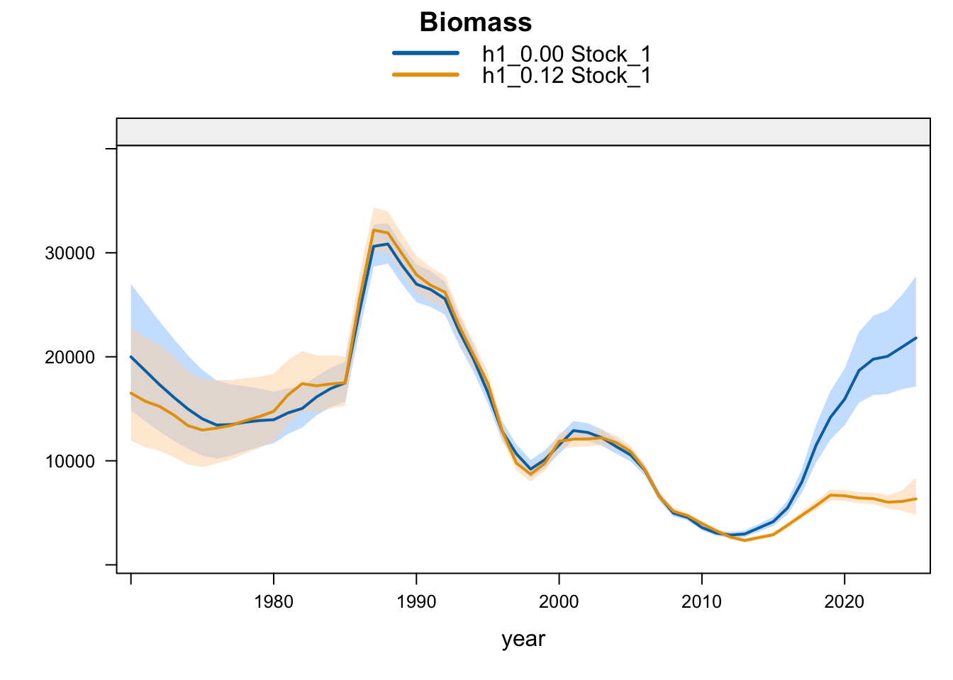
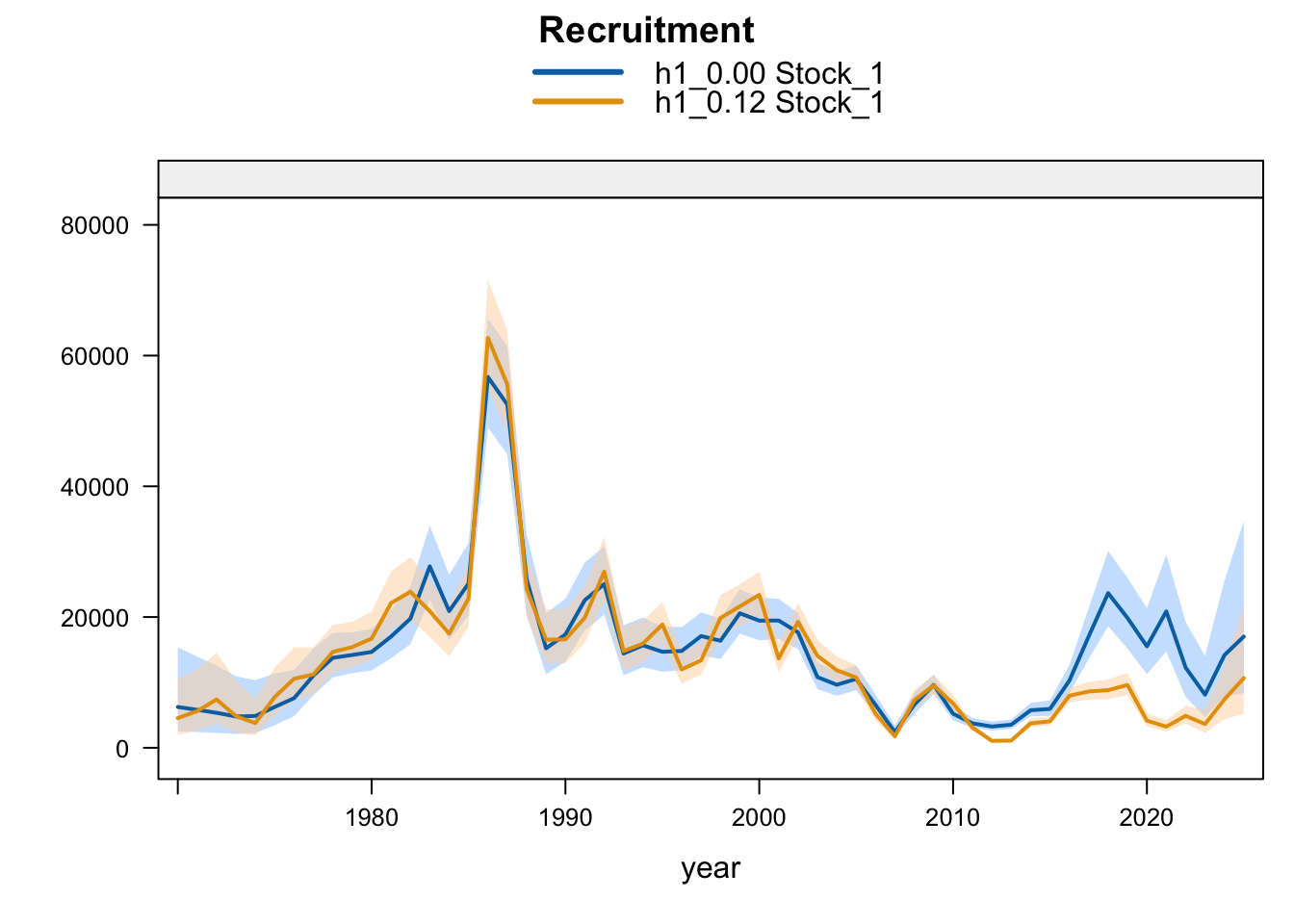
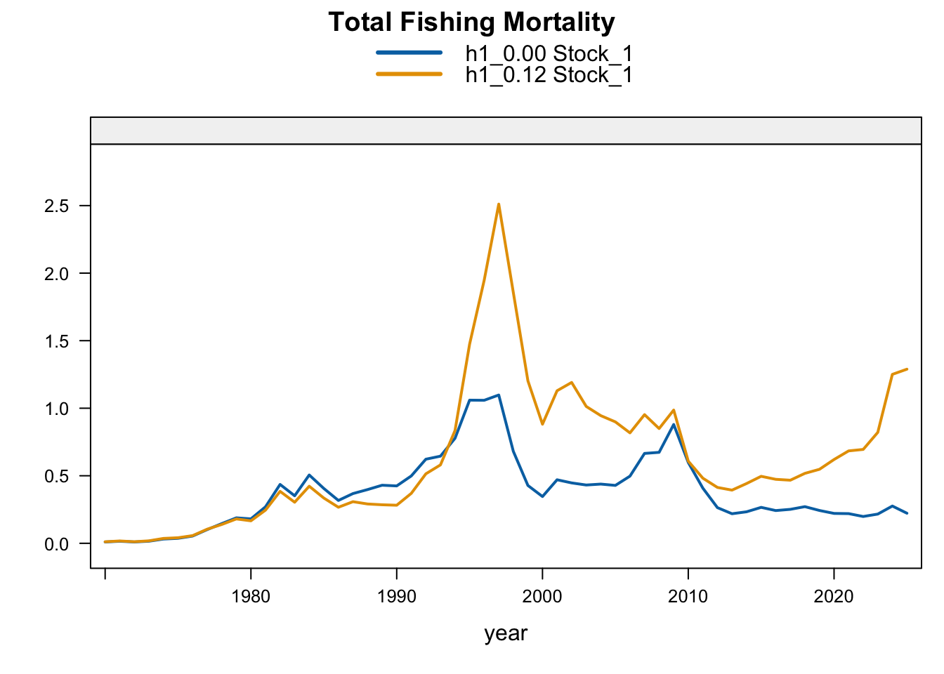
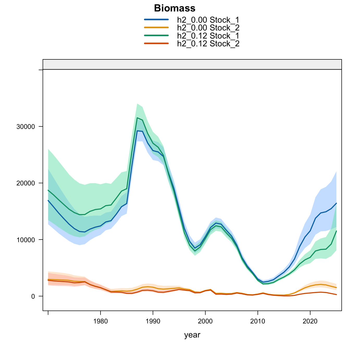
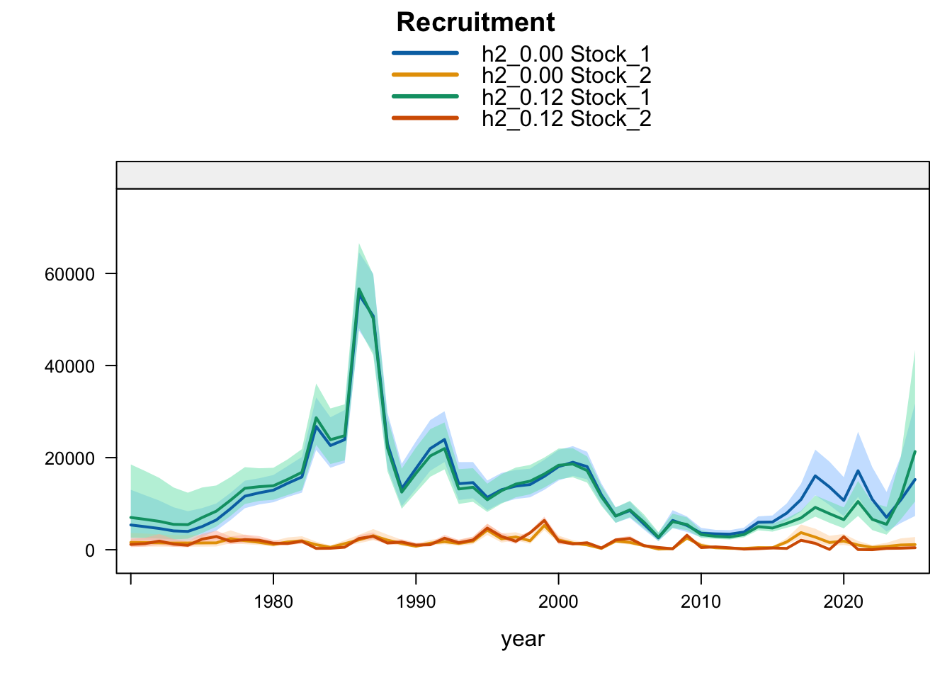
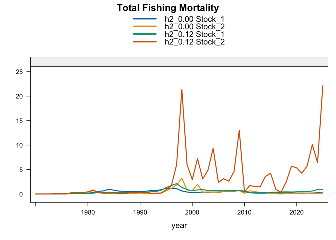
Model 0.12 is the previous final bridge configuration and model 0.14 is the proposed final configuration used for diagnostics in this report. The plots below compare the 0.00 SC13 baseline, 0.12, and proposed final 0.14 for each stock-structure hypothesis.
5.1 Single-Stock Hypothesis
5.2 Two-Stock Hypothesis
6 Final Model Diagnostics
The diagnostics below use model 0.14 as the proposed final model. Model 0.14 starts from 1.03, which drops the two seasonal Peru acoustic abundance-index series (Peru_Acoust_S1 and Peru_Acoust_S2), and adds the same 2018 Peruvian CPUE catchability break used in 0.13. Retrospective diagnostics use the standard five peels completed for 0.14.
6.1 Single-Stock Hypothesis
For the single-stock proposed final model, the diagnostics are interpreted as evidence about the internally aggregated stock trajectory. The main diagnostic tension is expected in recent composition and index data because 0.14 removes DEPM, drops the two seasonal Peru acoustic series, and relies on the remaining fishery, acoustic, and CPUE information to resolve the recent scale and age/length structure.
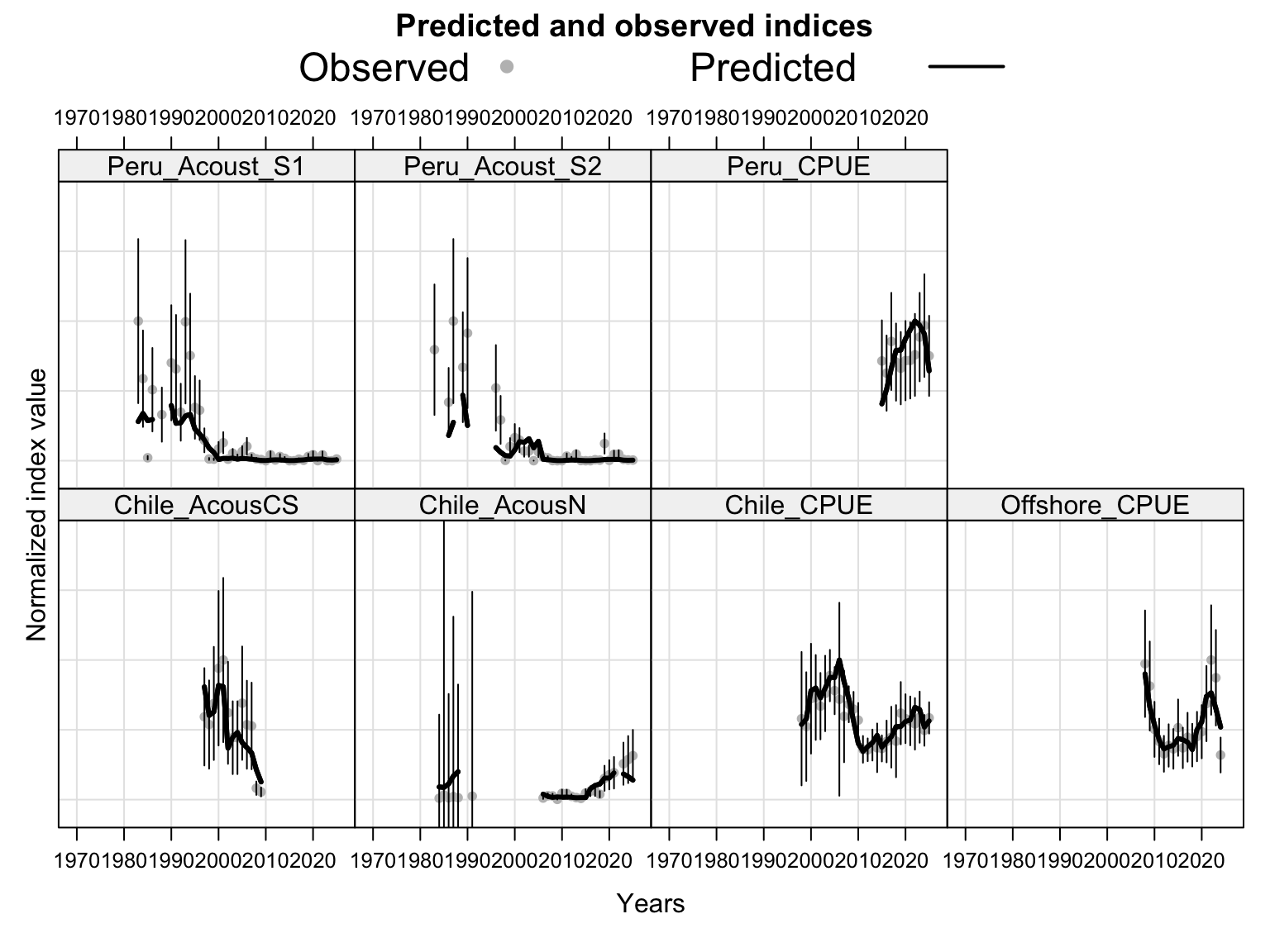
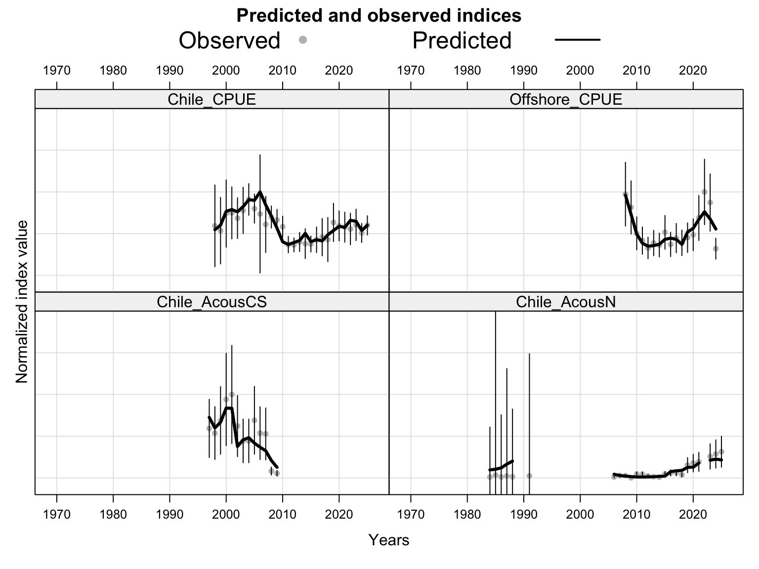
The index fits provide the primary check on whether the proposed final model follows the retained abundance-index signals after dropping DEPM and the seasonal Peru acoustic series. The single-stock model fits a common population trajectory to all retained indices, so departures among individual series should be read as conflicts in relative scale and timing rather than as stock-specific deviations.
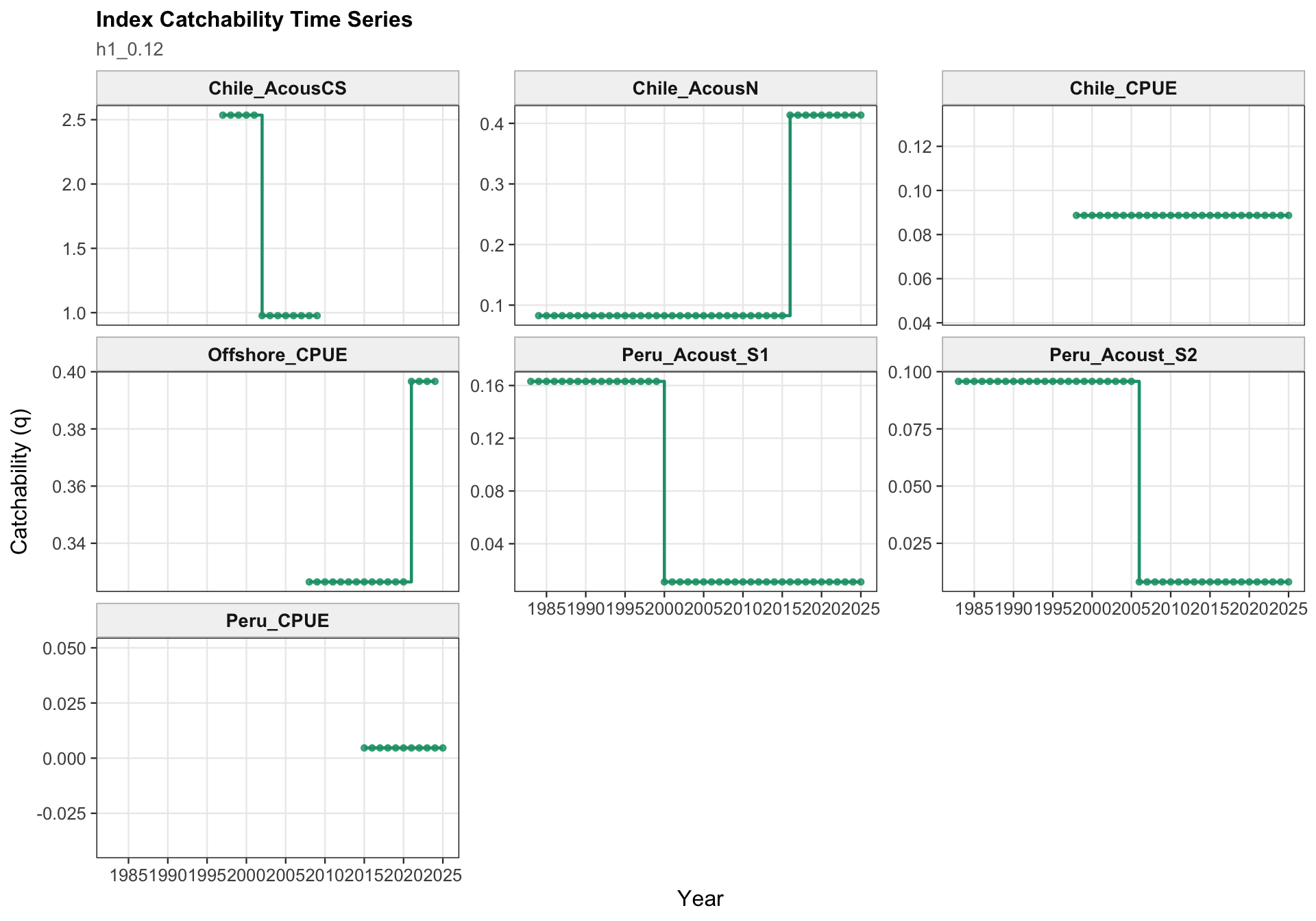
The catchability time series show the fitted q path used to scale vulnerable biomass to each retained abundance index. Step changes identify indices with block-specific or time-varying catchability estimates, while flat segments indicate periods sharing the same catchability estimate.
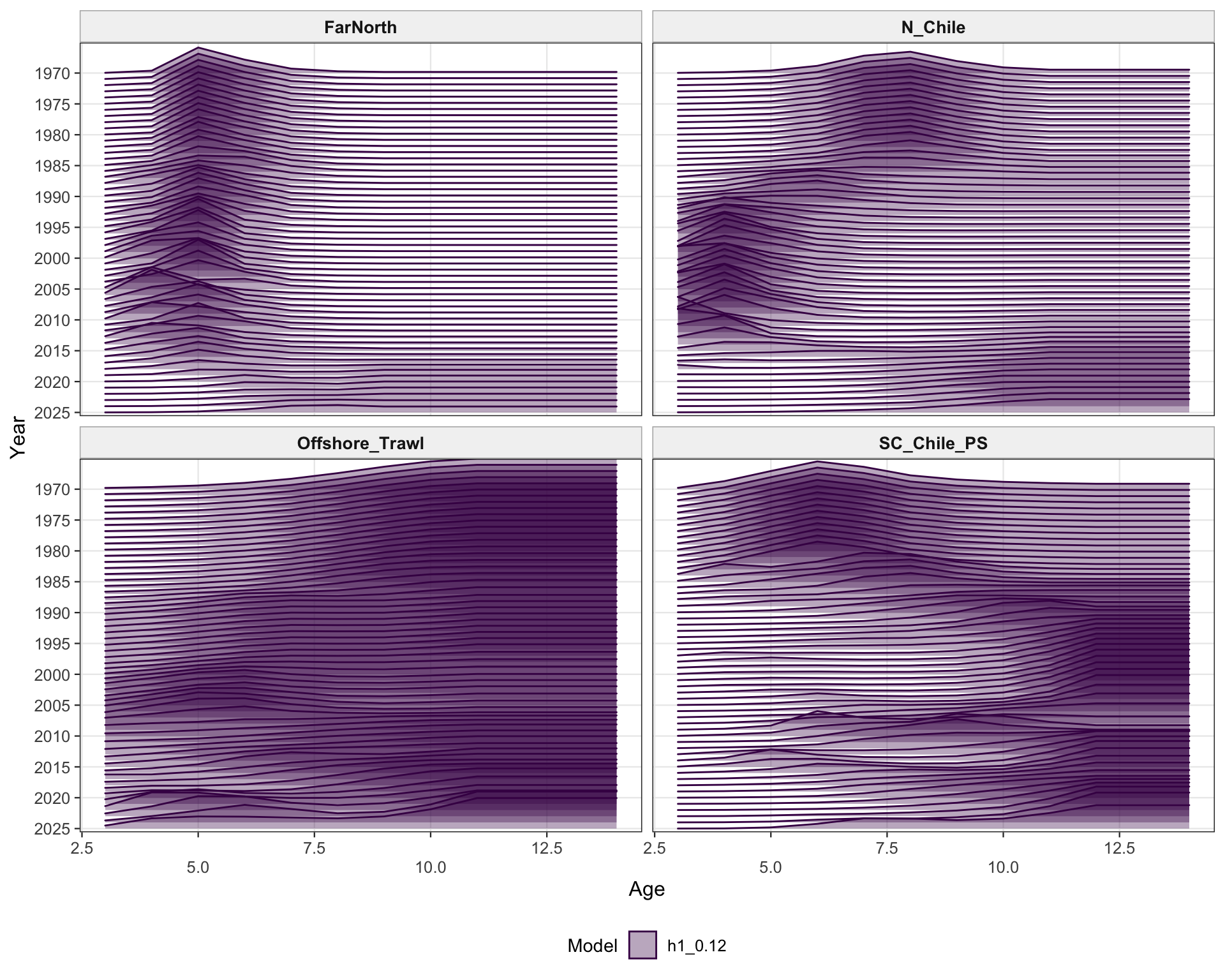
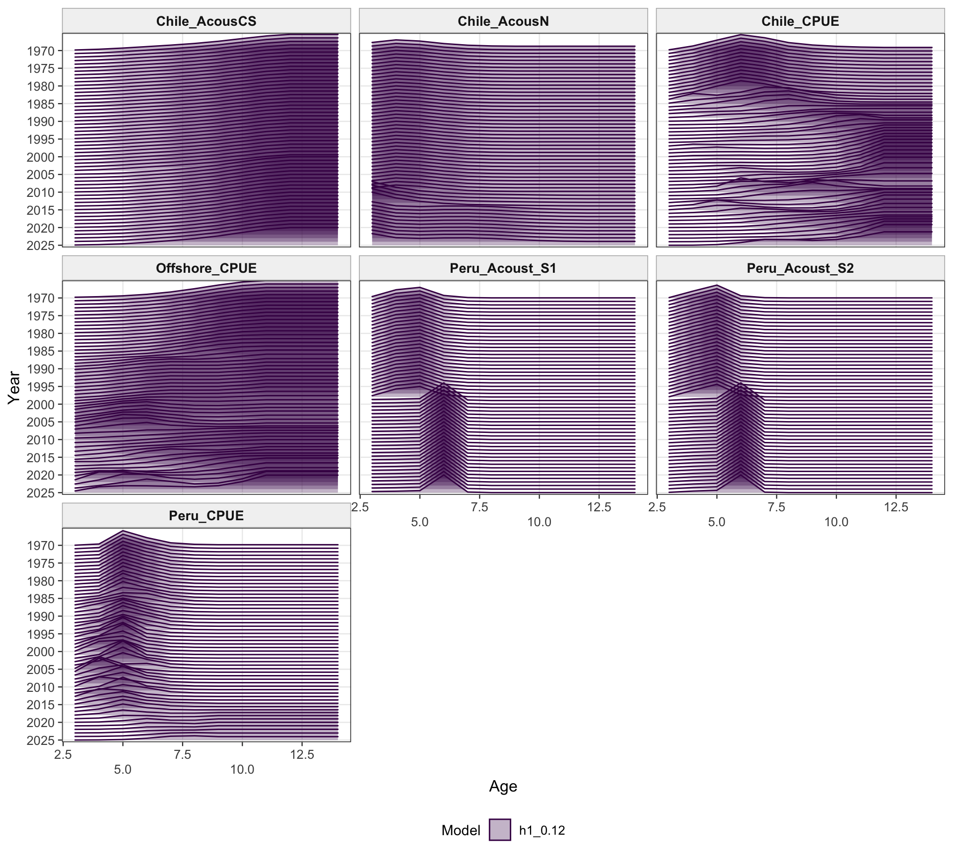
The selectivity plots show the time-varying age pattern that links each fishery and survey/index series to the modeled population. For the single-stock model, the fishery panel shows the strongest temporal changes in the FarNorth and Chilean fisheries, while the survey/index panel shows the selectivity assumptions used for acoustic and CPUE index observations. These plots are included as selectivity diagnostics; CPUE series remain relevant here even though CPUE age weights are not treated as age-composition fits below.
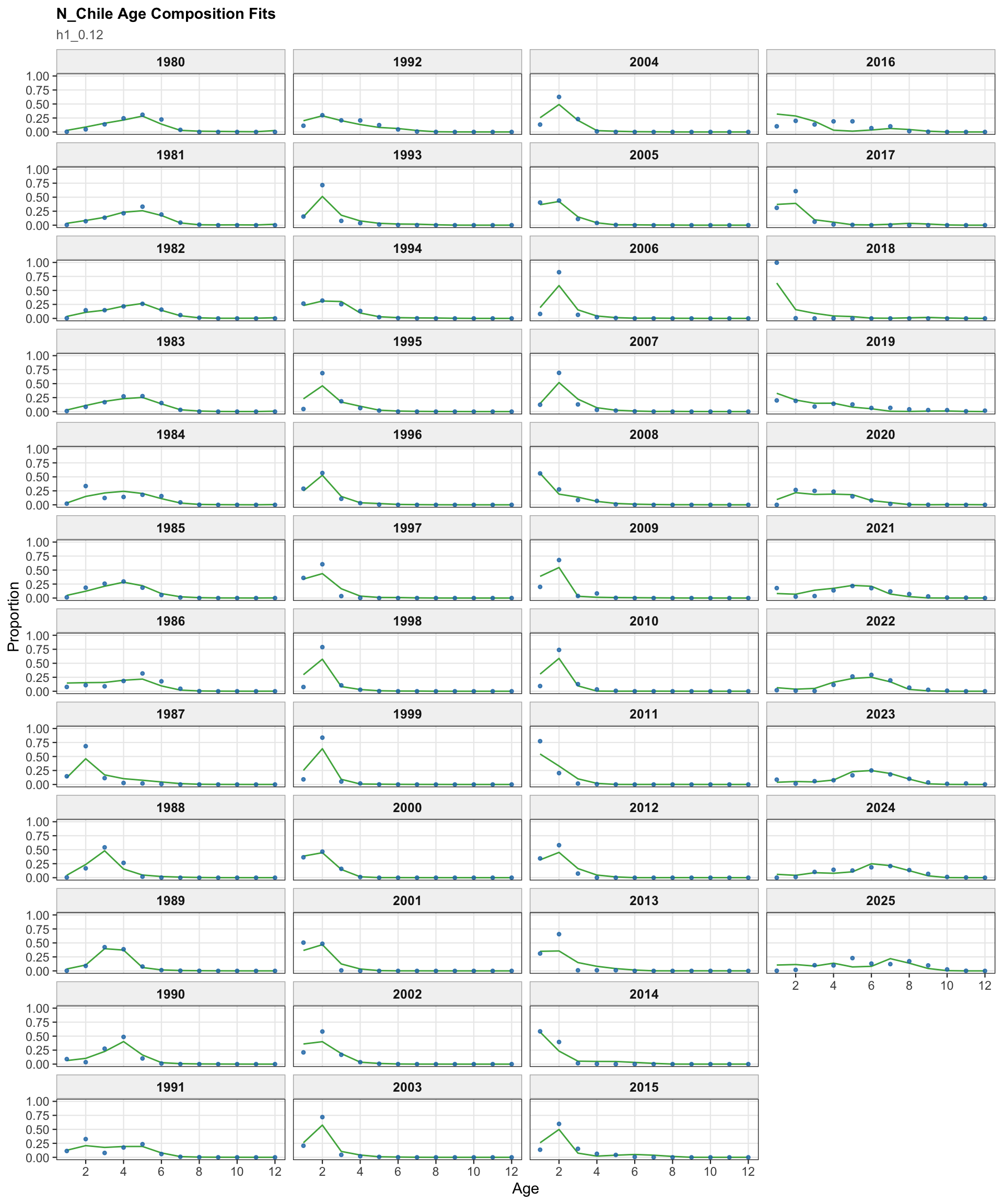
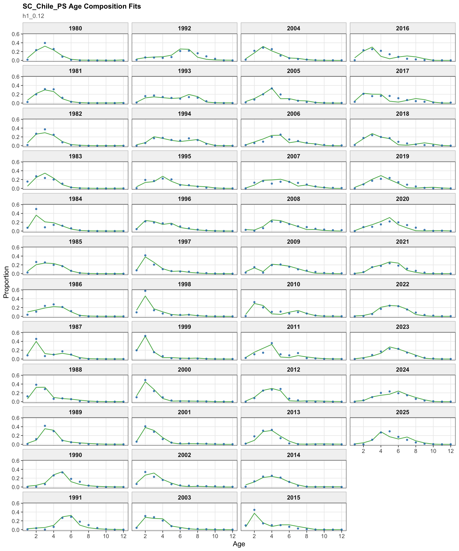
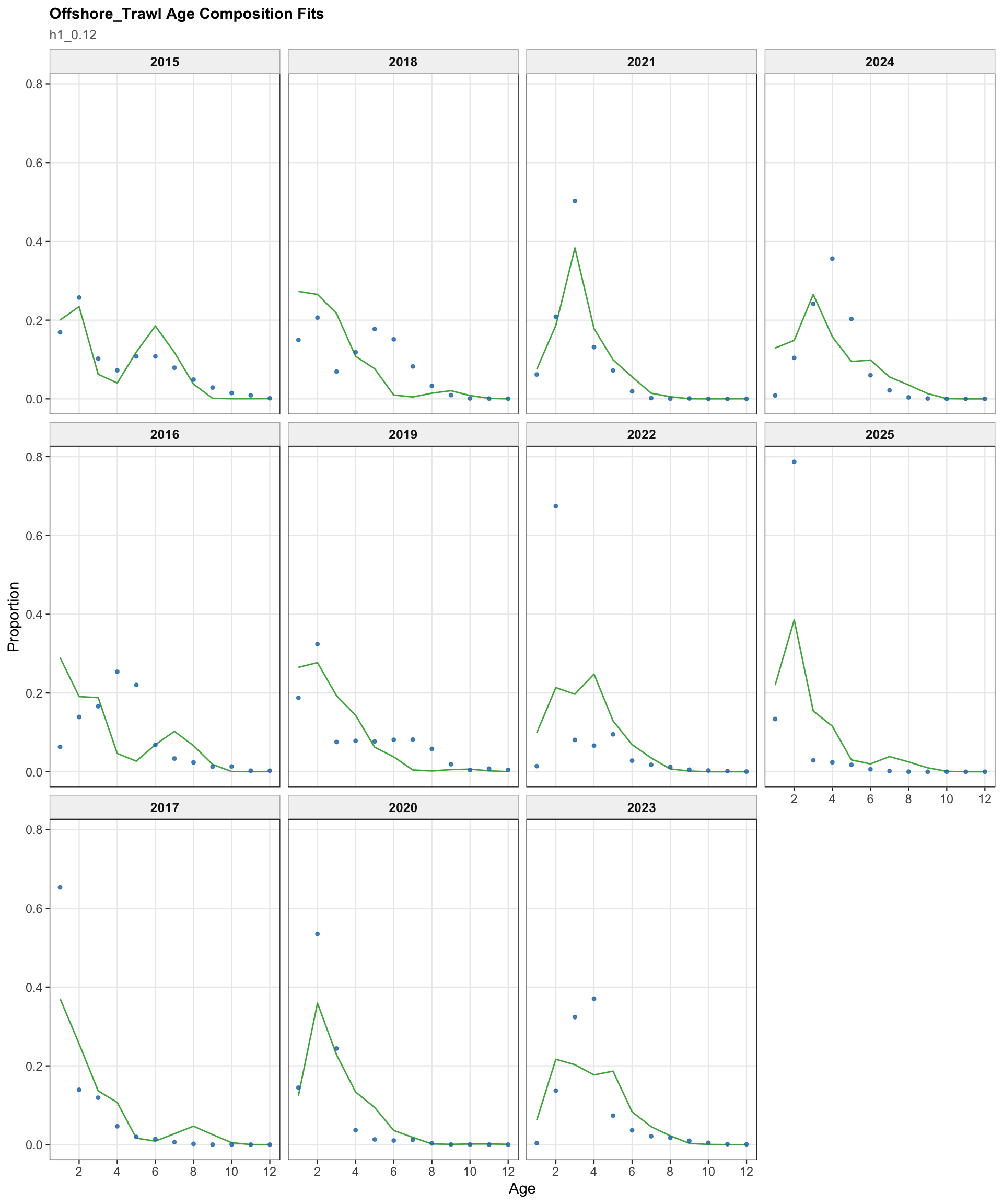
The fishery age-composition plots show the proposed final model tracking the main modal shifts in the Chilean and offshore-trawl age data. The corrected ggplot panels keep each fishery separate; this avoids mixing the northern Chile, south-central Chile purse-seine, and offshore-trawl observations and makes the recent modal ages easier to compare among fleets.
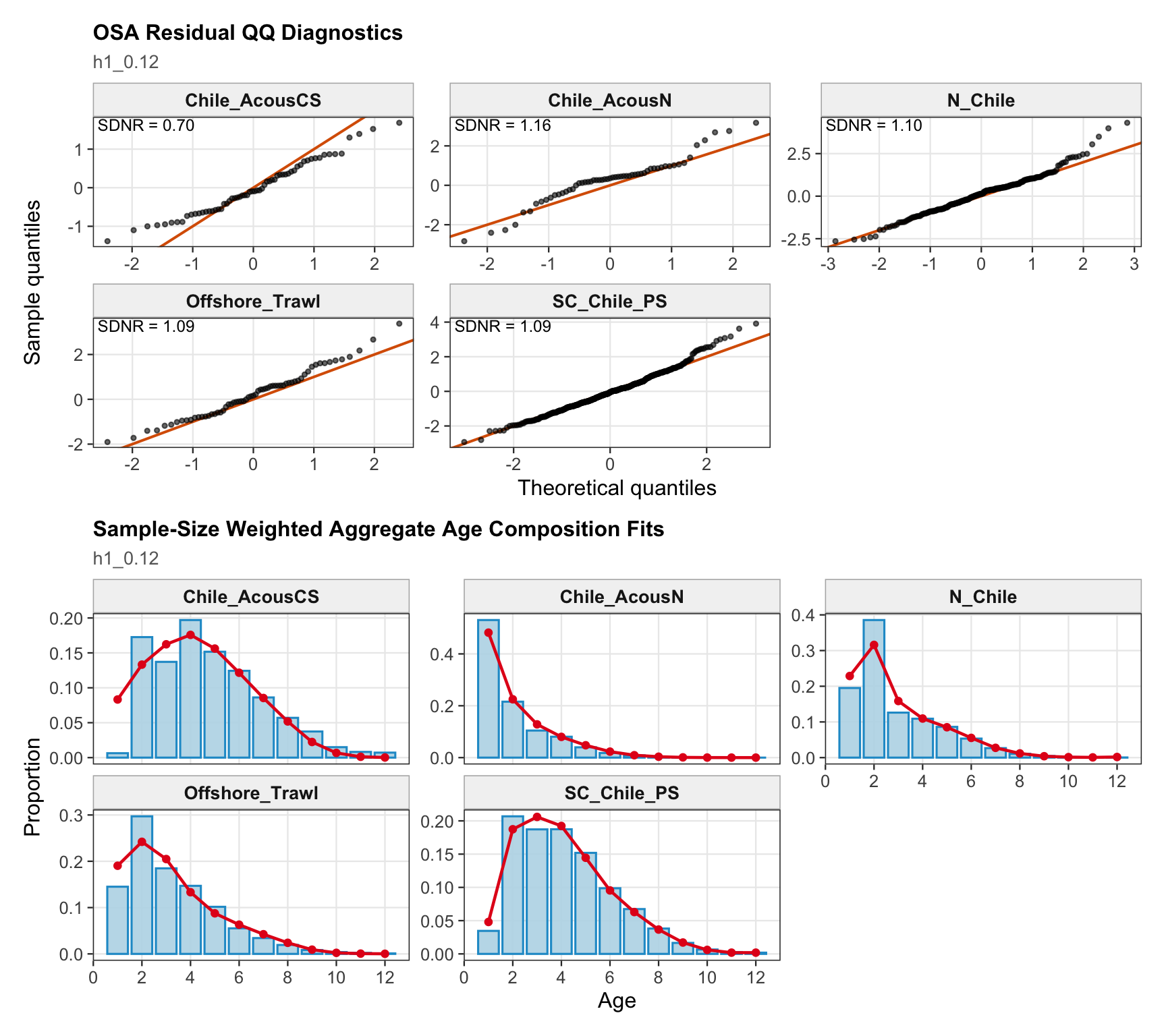
The OSA and aggregate age-composition diagnostics summarize the non-CPUE age-composition fits at a coarser level. They include the fishery age compositions and the acoustic-survey age compositions available in the proposed final model output, such as the central-south and northern Chile acoustic series. CPUE-index age weights are excluded here because they are not interpreted as age-composition observations for this diagnostic.
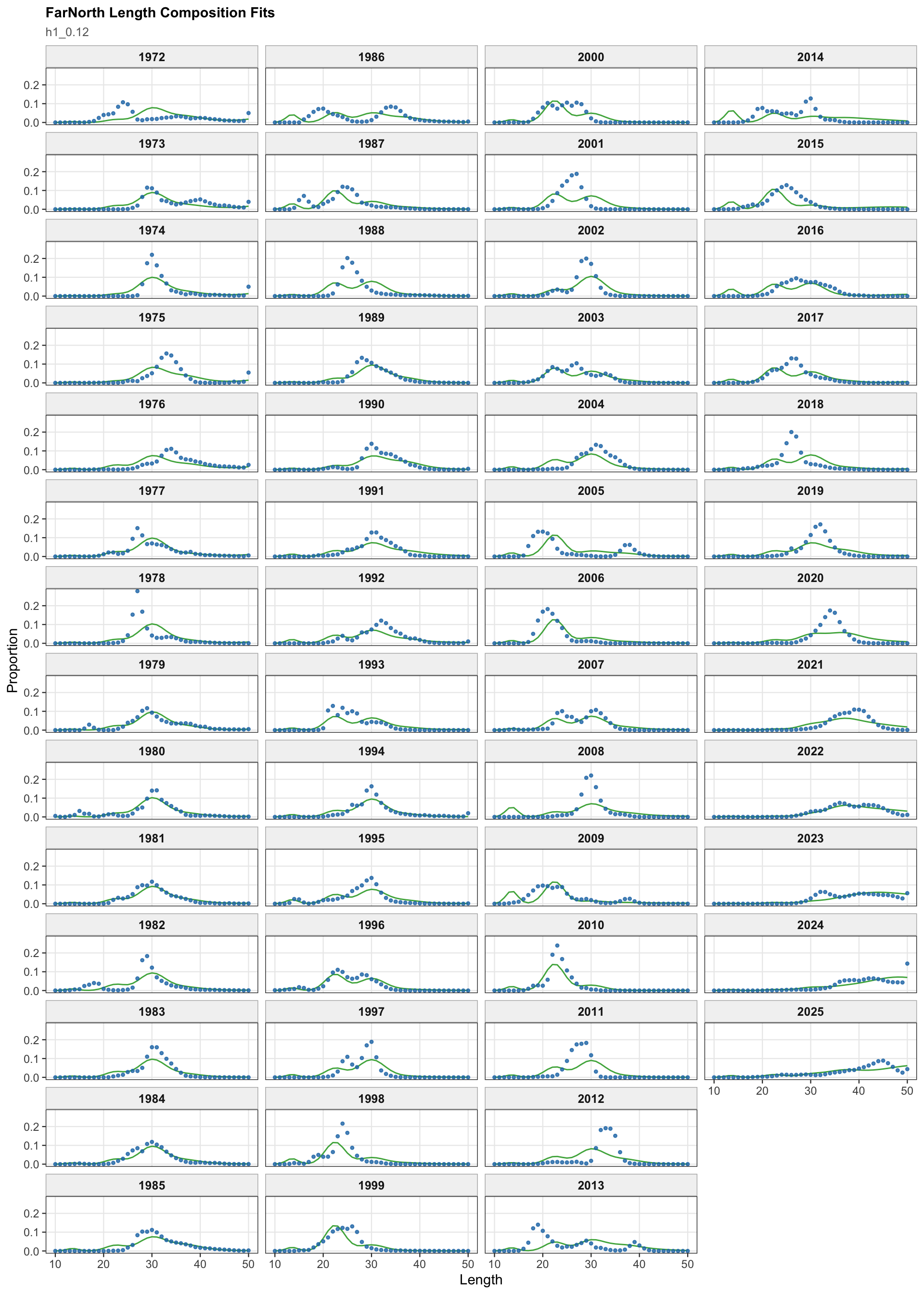
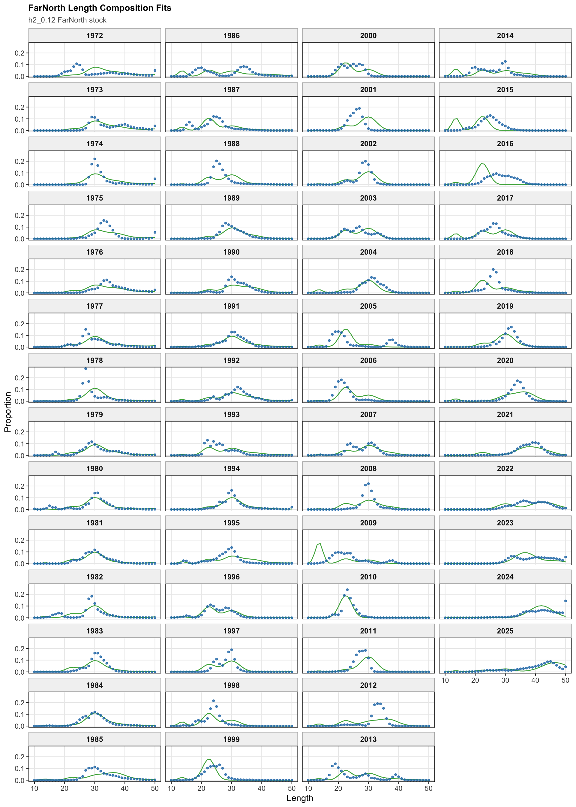
The FarNorth fishery length-composition panels now use the same observed-point and predicted-line style as the age fits. This makes the model fit to the long FarNorth length series easier to scan by year, particularly in years with narrow observed modes or sparse tails.
The length-composition OSA and aggregate diagnostics are limited to the FarNorth fishery for 0.14, because the two seasonal Peru acoustic length-composition series are not present in this proposed final configuration. These diagnostics show whether the broad residual pattern is concentrated in the retained fishery length data after the year-by-year panels are collapsed.
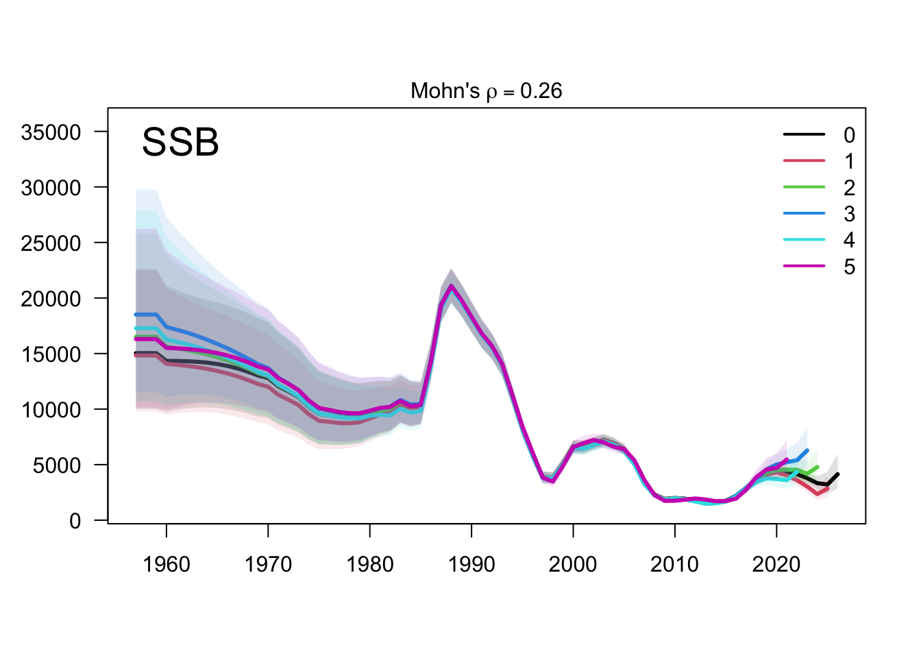
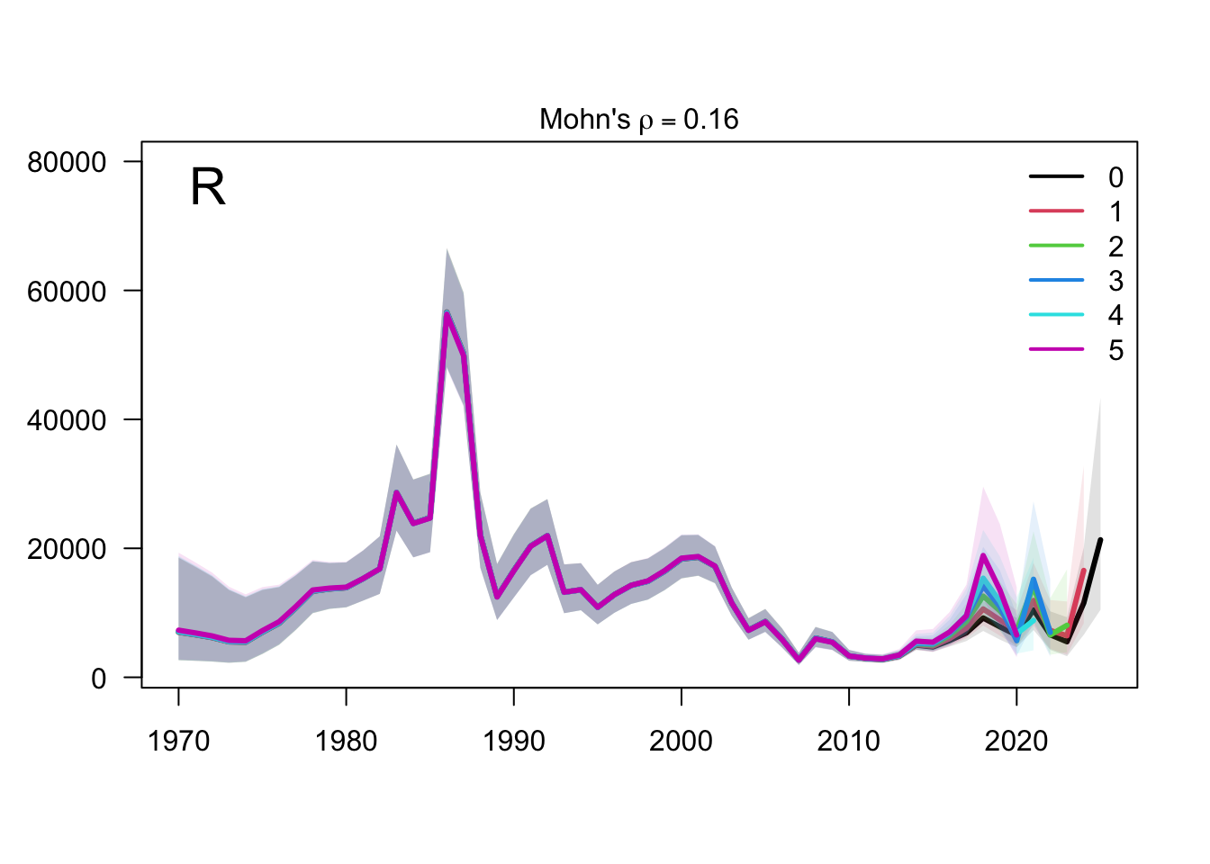
The retrospective SSB plot checks whether recent biomass estimates are stable when terminal years are peeled from the assessment. Any systematic peel pattern would indicate that the final years are exerting leverage on the single-stock biomass scale.
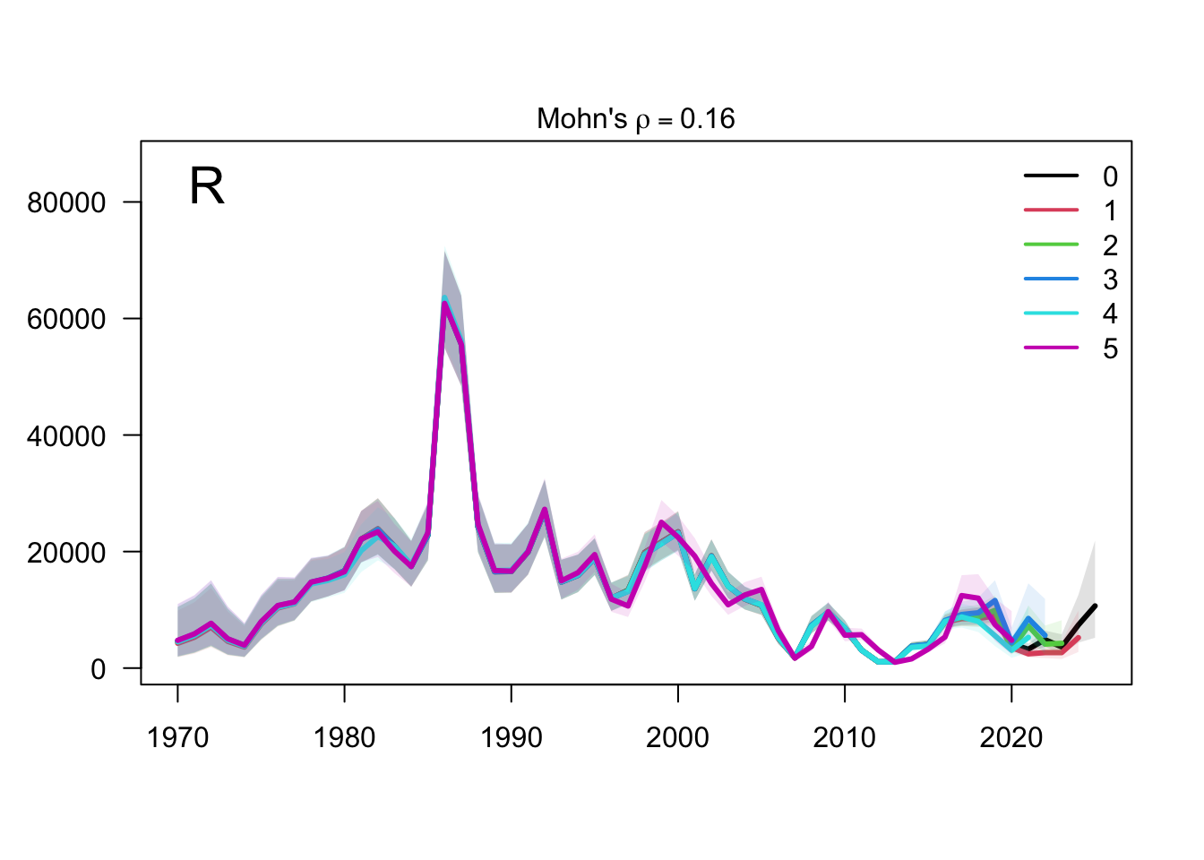
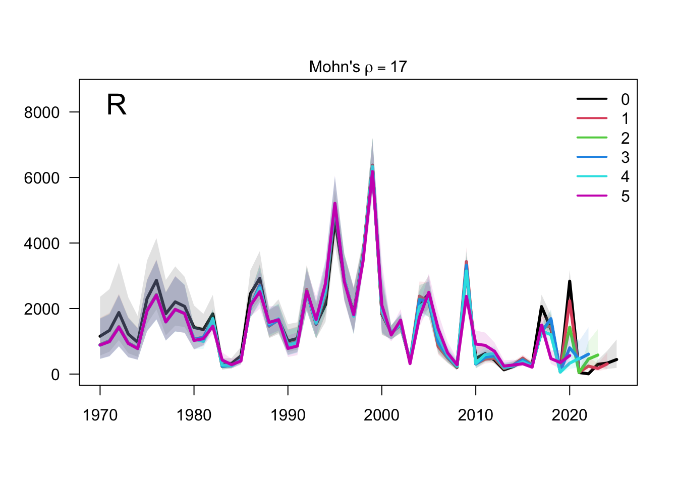
The retrospective recruitment plot provides the corresponding check for year-class estimates. Recruitment peels are expected to be more variable than biomass peels, but persistent directional changes would be evidence that recent data are revising the estimated strength of terminal cohorts.
6.2 Two-Stock Hypothesis
For the two-stock proposed final model, diagnostics are interpreted by stock. The southern stock carries the age-composition information, while the FarNorth stock carries the retained FarNorth fishery length-composition information and the Peruvian CPUE index. This split is important when comparing the diagnostic behavior with the data sensitivities because several sensitivity runs affect the FarNorth stock without changing the southern-stock trajectory.
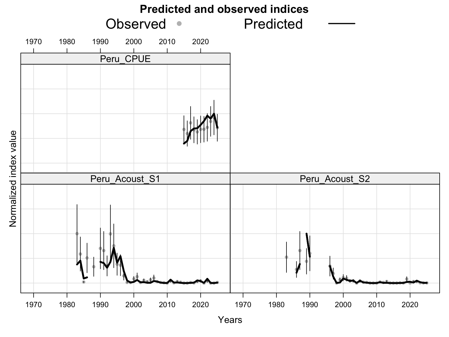
The two-stock index fits show how the proposed final model partitions retained abundance indices between the southern and FarNorth stocks. The FarNorth index behavior is especially important because 0.14 was proposed to relax the very low FarNorth biomass and high fishing-mortality behavior seen in the previous final bridge model, while keeping the Peruvian CPUE information with a post-2018 catchability break.
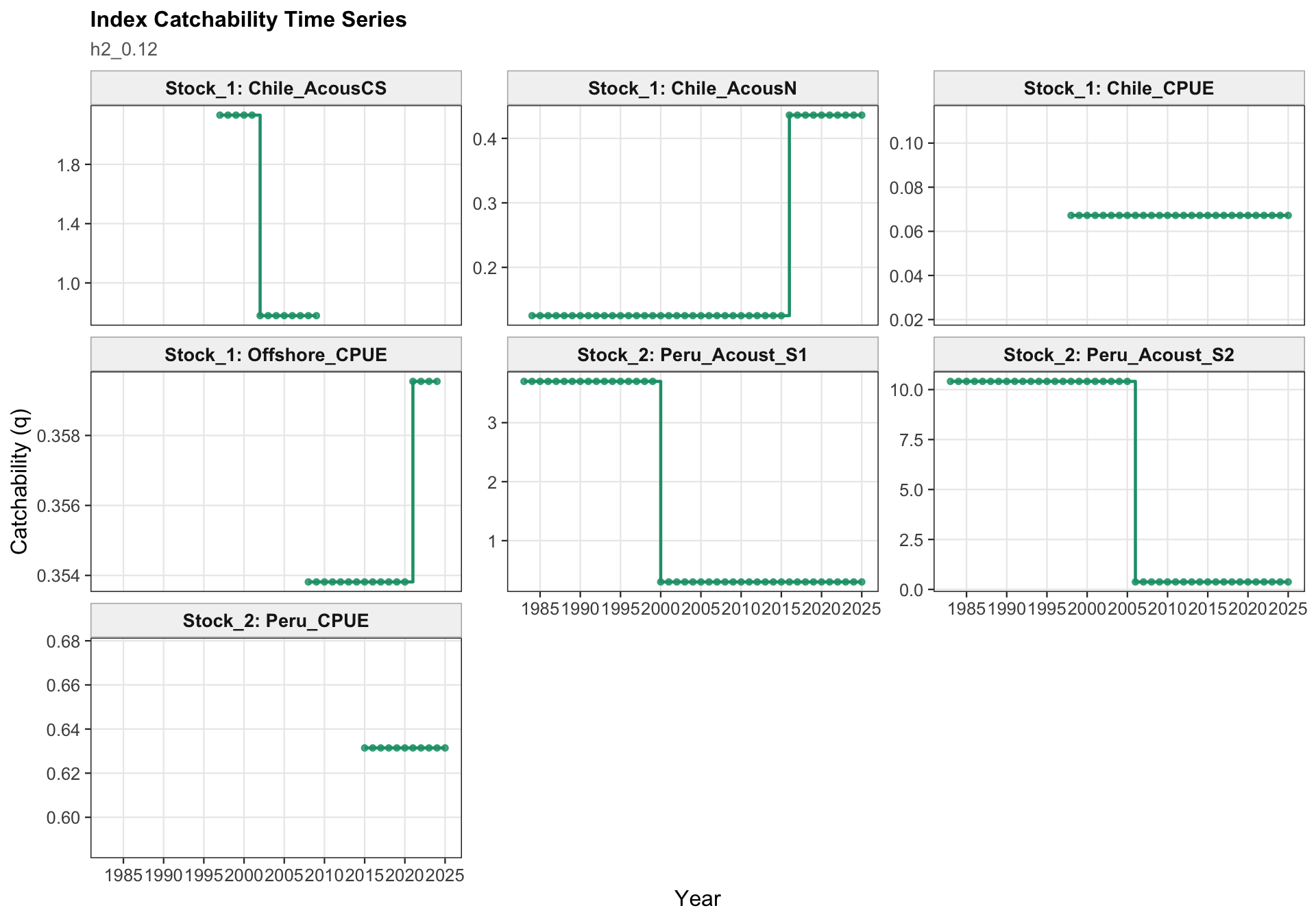
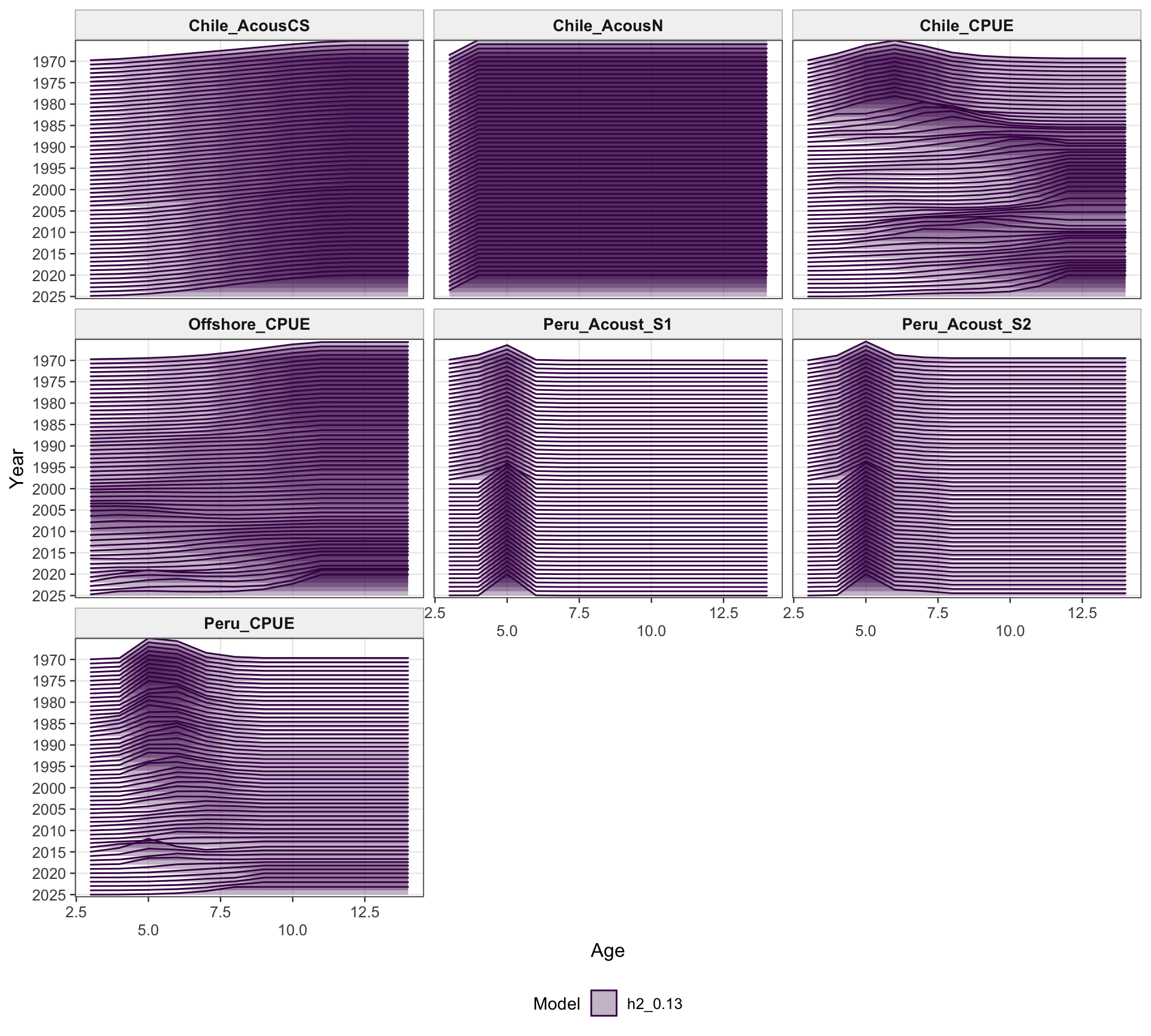
The two-stock catchability time series show which abundance-index catchability estimates apply to each stock. This panel is useful for checking whether the final configuration is using fixed or stepped catchability paths for the southern-stock and FarNorth-stock indices.
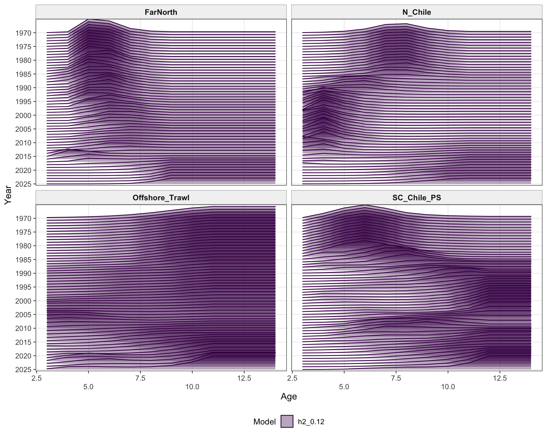
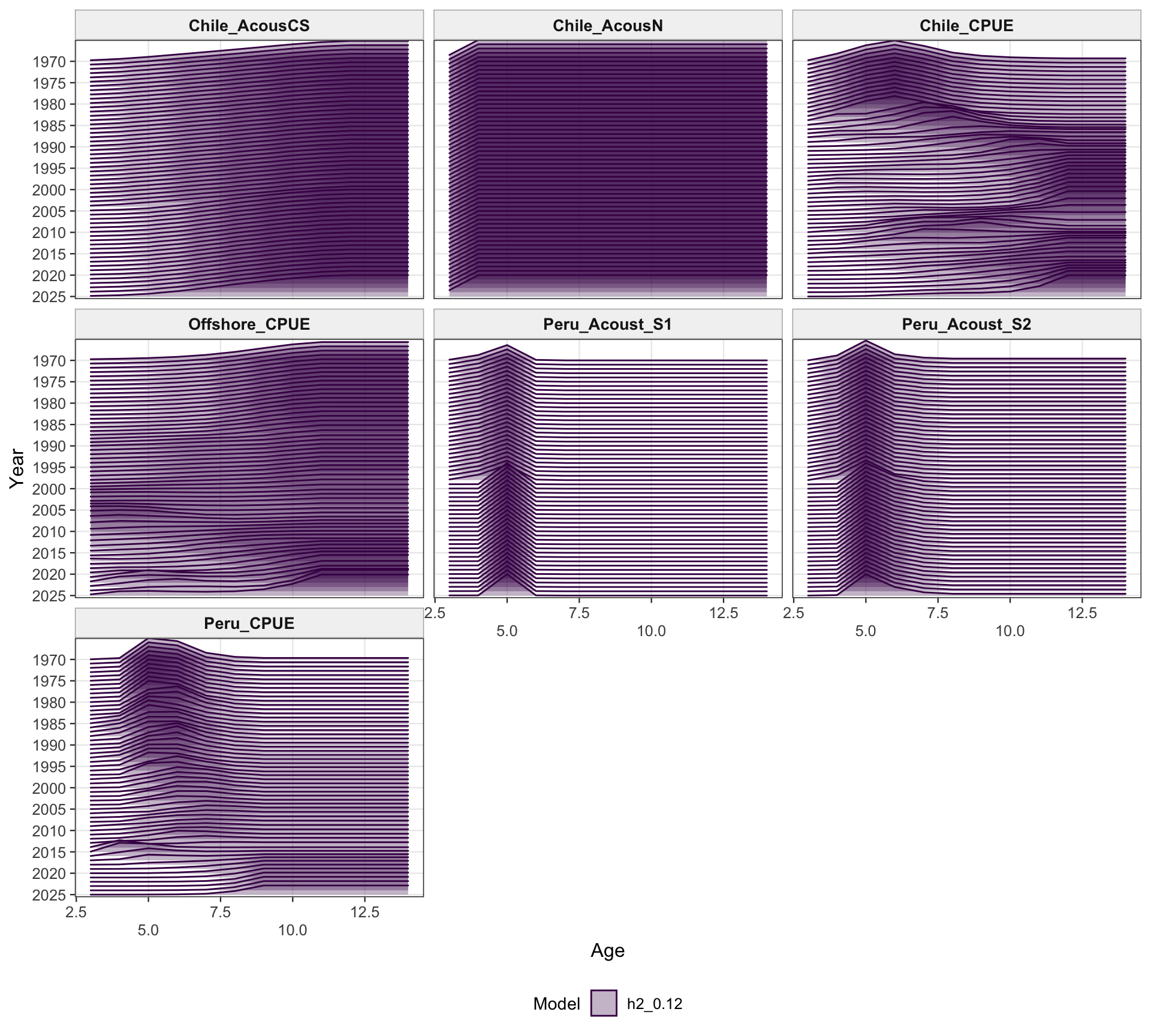
The two-stock selectivity plots separate the southern-stock fleets from the FarNorth fishery and survey/index selectivities. The fishery panel emphasizes the different selectivity structure assigned to the southern Chilean/offshore fisheries and the FarNorth fishery, while the survey/index panel shows the corresponding acoustic and CPUE selectivity patterns used by the retained abundance indices. The seasonal Peru acoustic series are not present in 0.14, so the FarNorth length-composition diagnostics below focus on the FarNorth fishery.
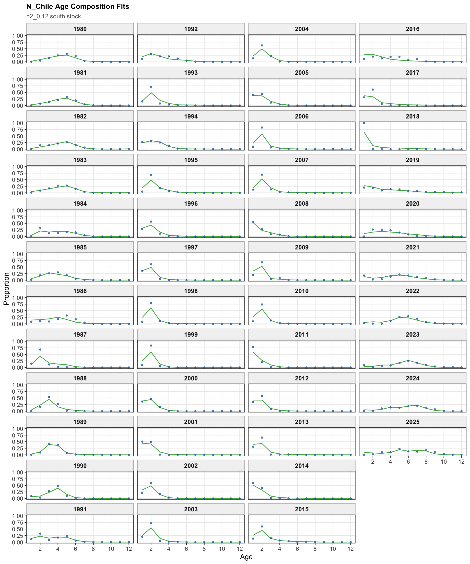
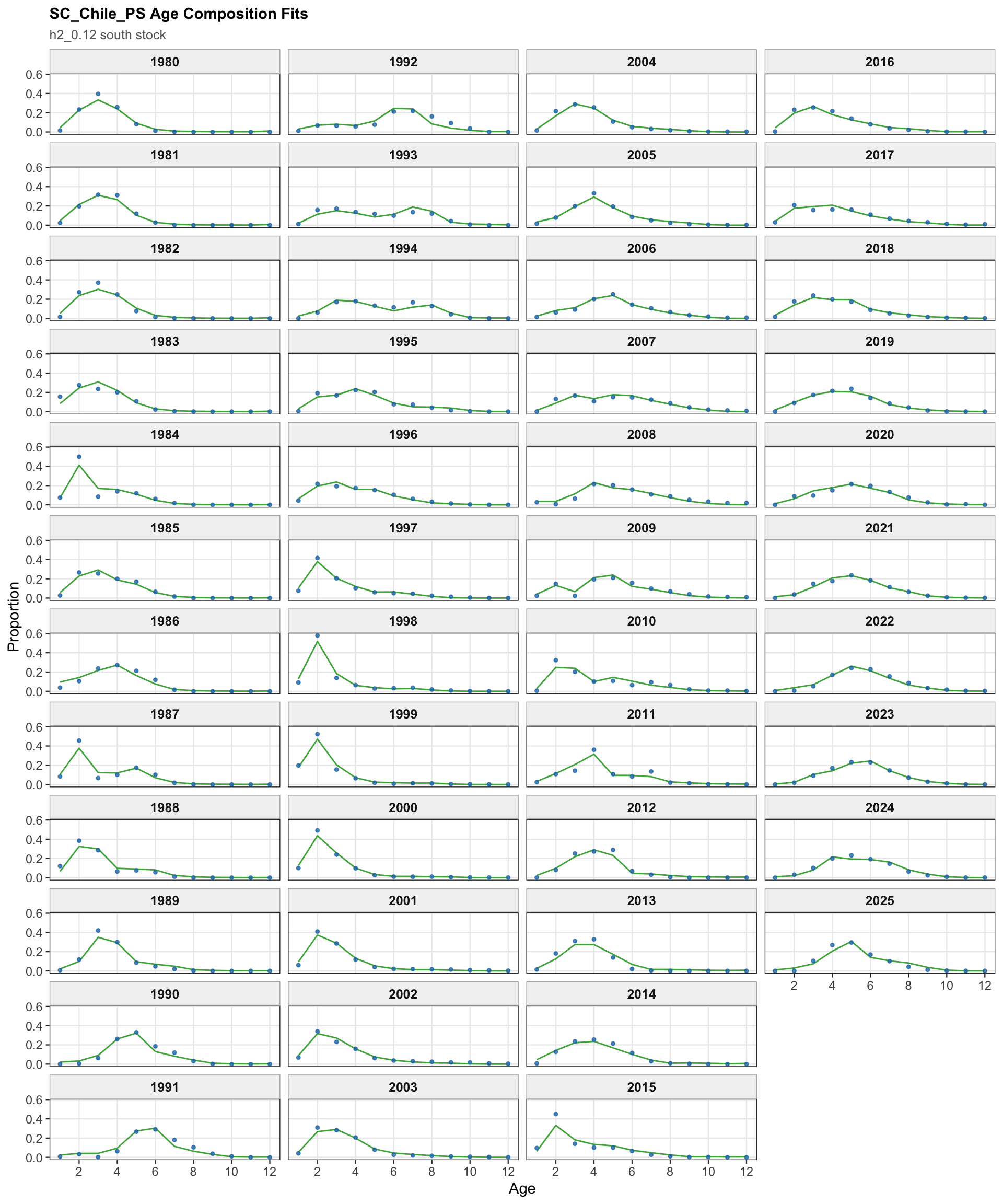
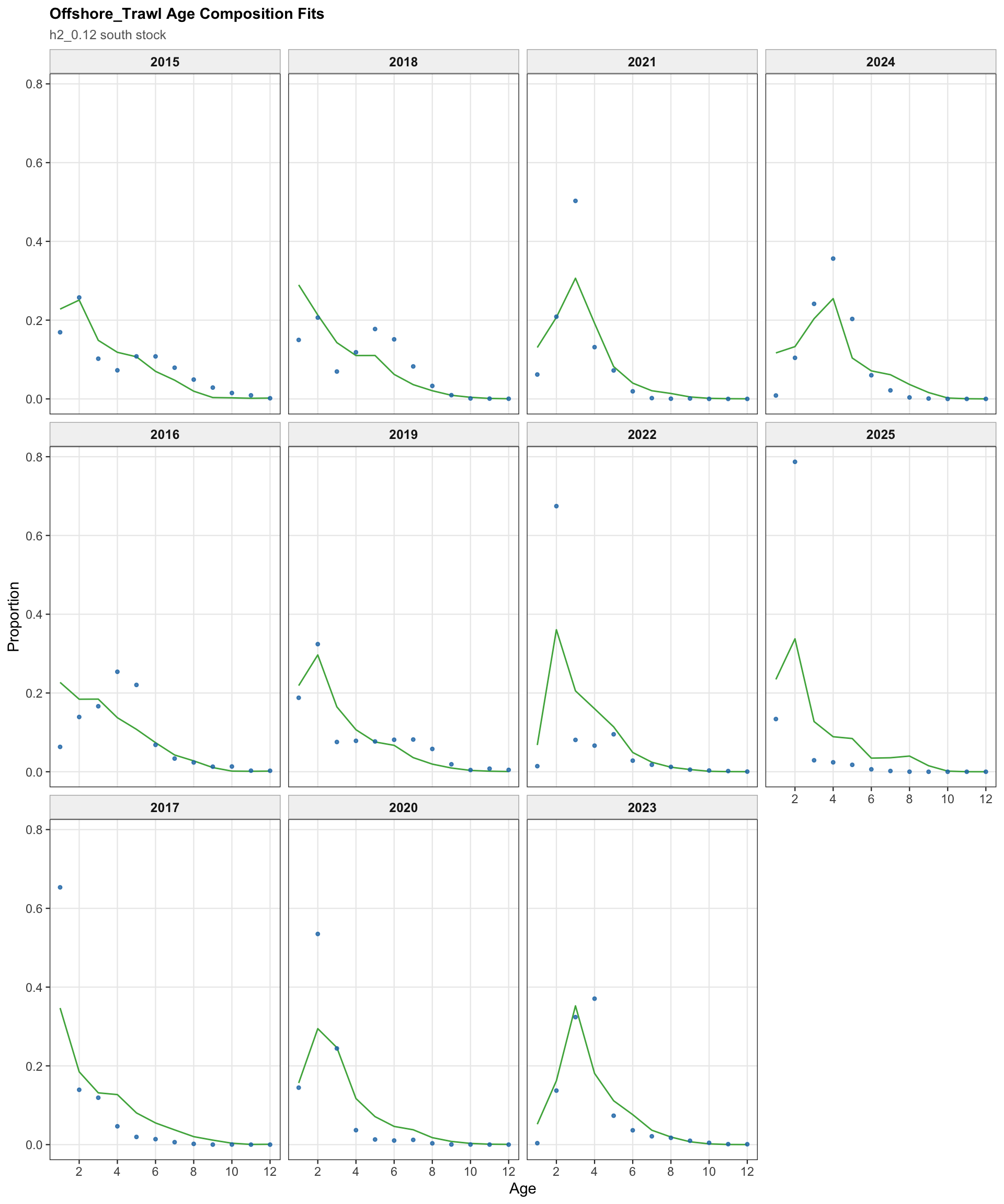
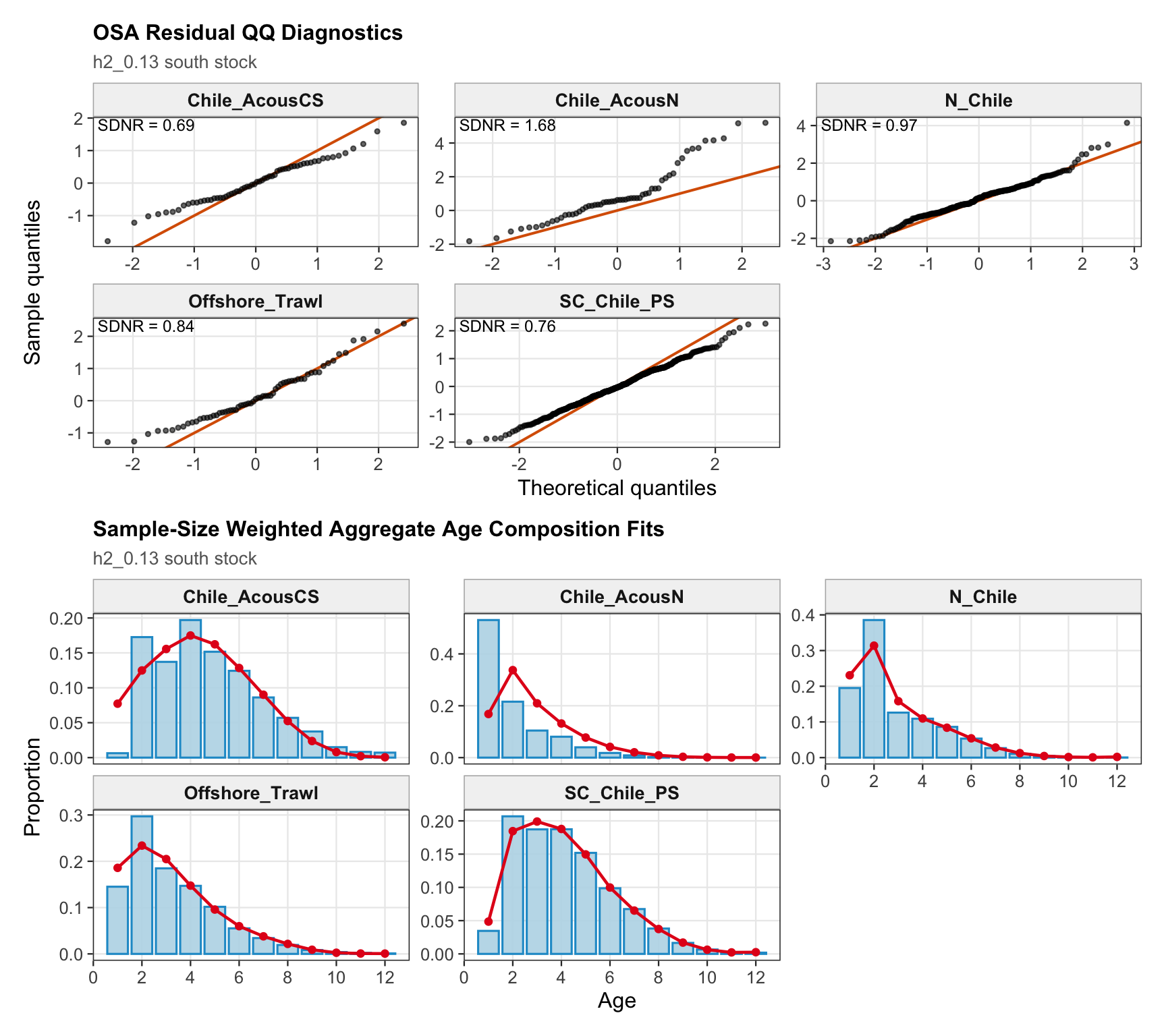
The age-composition diagnostics for the two-stock model apply to the southern stock. The same fleet-specific ggplot display is used here as in the single-stock model, which makes differences in modal age and tail behavior among the southern-stock fisheries easier to identify.
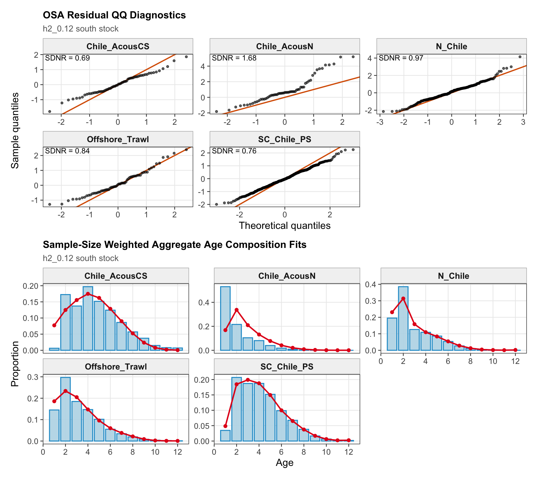
The OSA and aggregate age-composition diagnostics for the two-stock model summarize the southern-stock non-CPUE age-composition residuals. They retain the fishery age compositions and the Chilean acoustic-survey age compositions available for the southern stock, while excluding CPUE-index age weights. These diagnostics are complementary to the year-by-year age panels because they show whether residual departures are broadly distributed or concentrated in specific fleets, surveys, or ages.
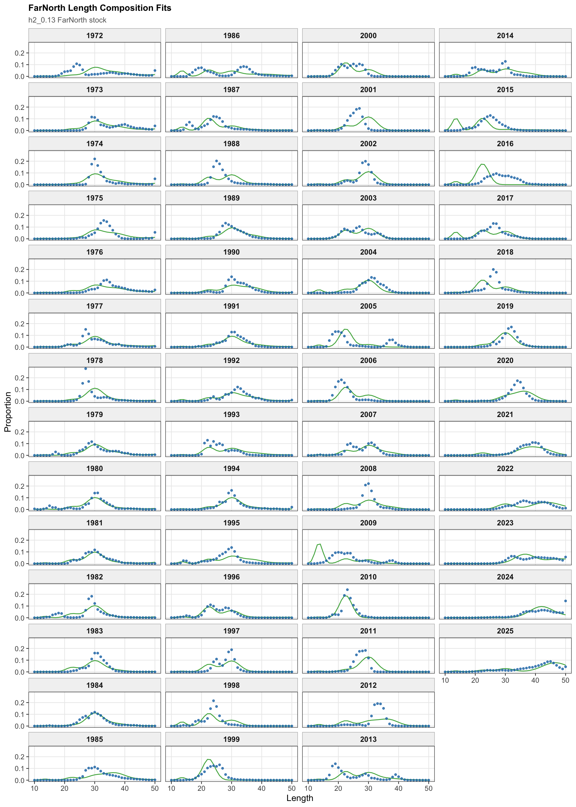
The FarNorth fishery length-composition diagnostics are shown on stock 2 for the two-stock model. These fits are central to evaluating the FarNorth component because the FarNorth terminal biomass and fishing mortality are highly sensitive to the treatment of Peruvian data.
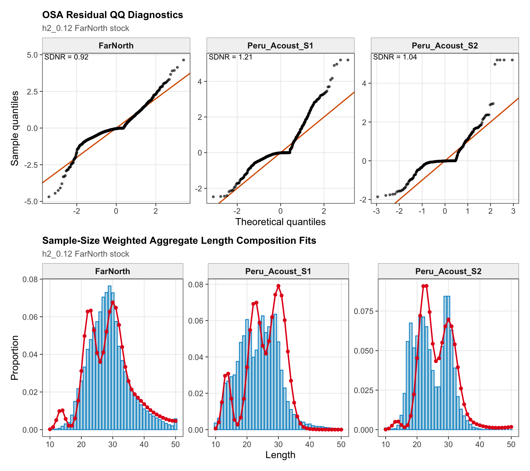
The FarNorth-stock length-composition OSA and aggregate diagnostics are limited to the FarNorth fishery for 0.14. This keeps the diagnostic aligned with the proposed final data configuration and avoids implying that the removed seasonal Peru acoustic length-composition series contribute to the run.
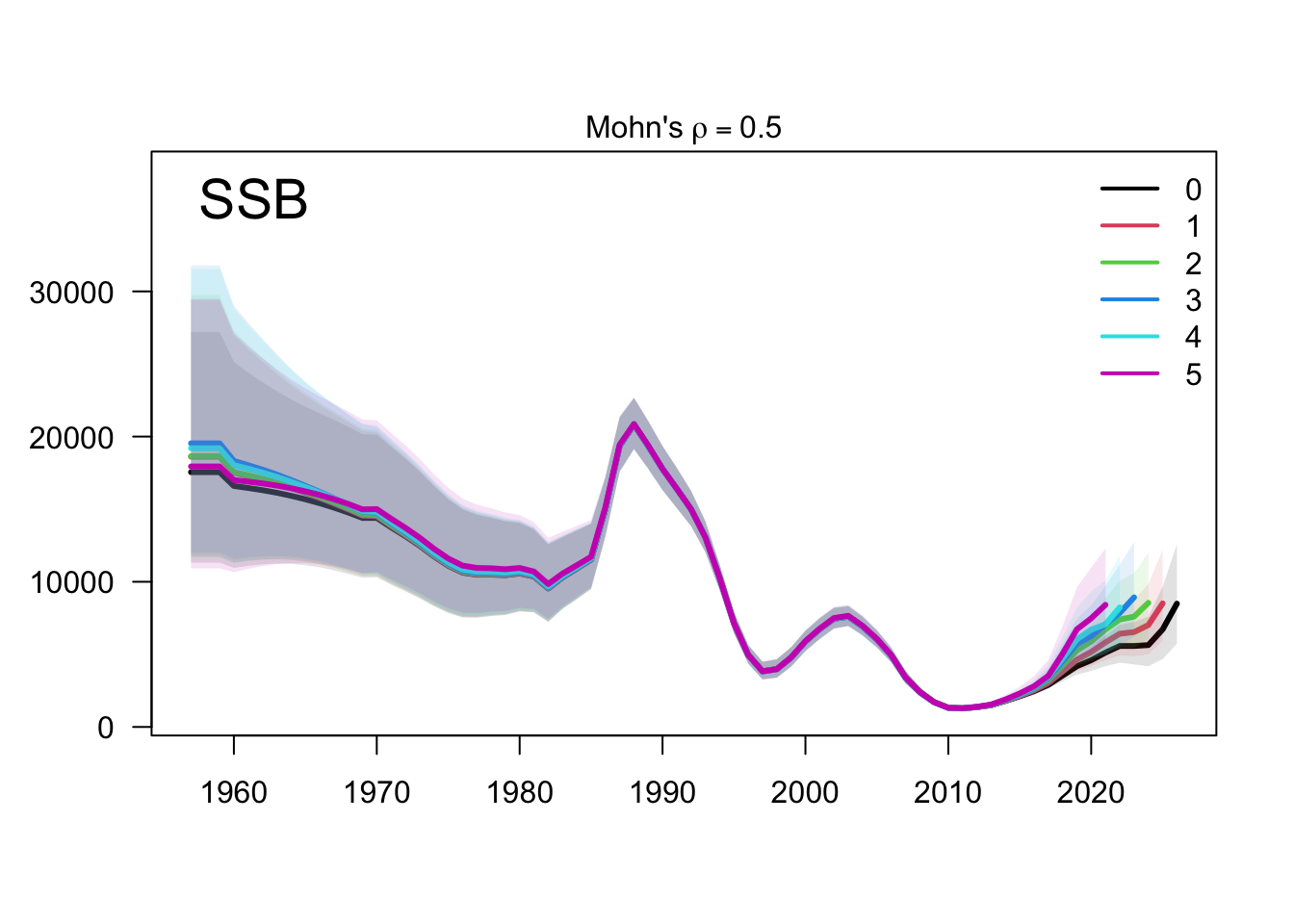
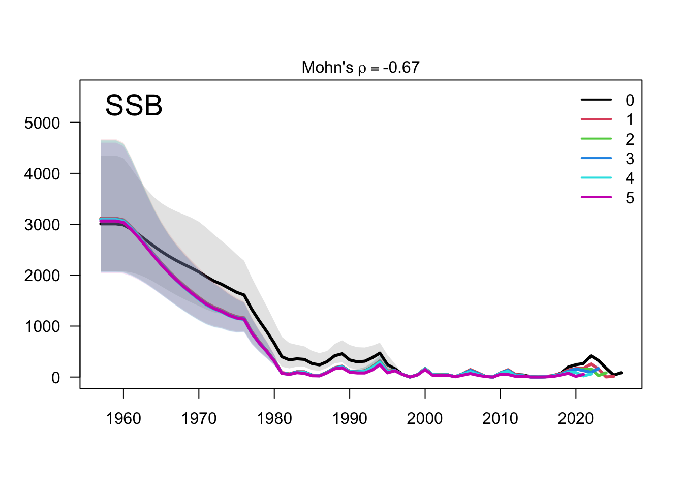
The two-stock retrospective SSB plot should be read by stock because peel behavior can differ between the southern and FarNorth components. The FarNorth trajectory is the key diagnostic target because the proposed final model changes the Peruvian/FarNorth data treatment relative to the previous final bridge configuration.
The two-stock recruitment retrospectives evaluate whether recent year-class estimates are stable under the same five peels. As with biomass, the FarNorth recruitment estimates should be interpreted alongside the data sensitivities because the composition and abundance-index information for that stock is more limited and more influential.
7 ADNUTS MCMC Diagnostics
ADNUTS MCMC diagnostics were not rerun after the latest two-stock 0.13 and proposed final 0.14 control-file updates. The deterministic fits, final-model diagnostics, and 0.14 retrospective diagnostics in this report use the updated runs, but MCMC diagnostics are intentionally omitted from this version.
8 Data Sensitivities
These sensitivities are shown against both the previous final bridge model (0.12) and the proposed final model (0.14). Most sensitivities were developed from the 0.12 bridge configuration; 1.04 starts from 1.03 and adds back the old Peru_Acoustic series from 0.00, while proposed final 0.14 starts from 1.03 and adds the same 2018 catchability break for the Peruvian CPUE index used in 0.13. Model 0.13 keeps the 0.12 data and adds only the 2018 Peruvian CPUE catchability break. For the two-stock hypothesis, the 0.12, 0.13, and 0.14 bridge comparisons reflect the latest updated control-file runs, while the earlier data-sensitivity outputs remain the completed trial runs shown for comparison. The terminal-year metric and percent-difference tables are provided near the beginning of the report and are not repeated here.
SC13_1.15 is included as an additional SC13-style sensitivity. It fully downweights the Acoustic N and Peruvian CPUE index series across all years, effectively removing their likelihood contribution rather than only reducing the influence of terminal-year observations. The run should therefore be interpreted as a diagnostic of how strongly those two complete index series affect the final-year stock status and fishing mortality pattern rather than as a competing final-model configuration.
8.1 Single-Stock Hypothesis
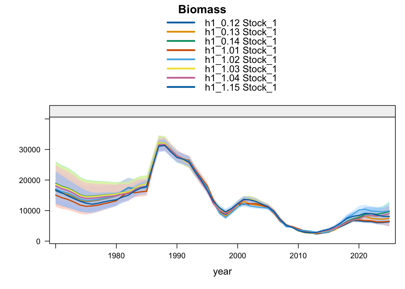
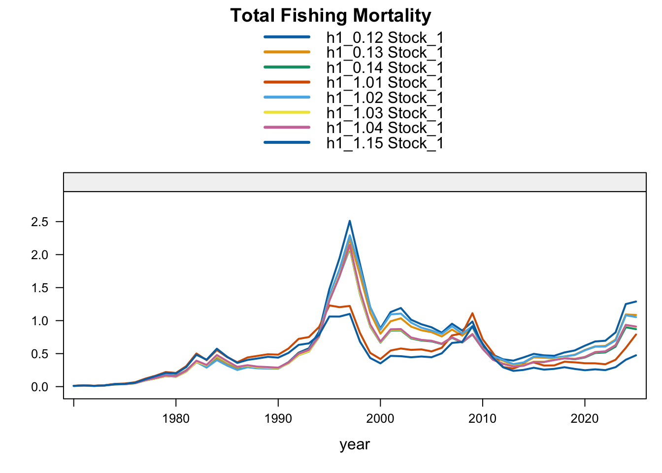
Under the single-stock hypothesis, the sensitivities retain the broad increase in biomass after the mid-2010s but differ in the magnitude of the rebuilding signal. Adding the 2018 Peruvian CPUE catchability break to the 0.12 data (0.13) raises terminal biomass relative to 0.12, but less than replacing the Peruvian CPUE (1.02) or dropping the two Peru acoustic series (1.03). Proposed final 0.14 applies the same catchability break after dropping the two Peru acoustic series, raising terminal biomass above 1.03 and leaving terminal fishing mortality below 0.12 but slightly above 1.03. Replacing the Chilean CPUE series (1.01) leaves terminal biomass close to 0.12, while adding the old Peru acoustic series back in 1.04 leaves the single-stock trajectory close to 1.03, indicating that the larger single-stock biomass response is driven mainly by removal of the two seasonal Peru acoustic series rather than by the replacement index itself. The SC13 downweighting sensitivity (SC13_1.15) is intermediate: terminal biomass is above 0.12 but below 1.02 and proposed final 0.14.
The biomass panel shows the strongest separation among single-stock sensitivities after about 2015. 1.02, proposed final 0.14, 1.03, and 1.04 all imply a higher recent biomass trajectory than 0.12, whereas 1.01 remains close to 0.12. The 0.13 catchability-break sensitivity and SC13_1.15 both give moderate upward shifts.
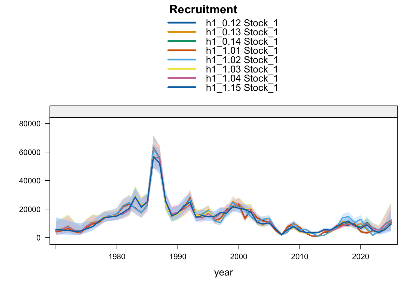
Recent recruitment remains elevated relative to the preceding low period across all single-stock sensitivities. The Peruvian CPUE and Peru acoustic sensitivities (1.02-1.04) produce somewhat higher terminal recruitment than 0.12; proposed final 0.14 is also higher because it combines removal of the two seasonal Peru acoustic series with the Peruvian CPUE catchability break. Model 0.13 is only slightly higher than 0.12, while SC13_1.15 gives lower terminal recruitment despite its higher terminal biomass.
The fishing-mortality response is not monotonic with biomass. 1.01 reduces terminal fishing mortality relative to 0.12, 0.13 and 1.02 increase it, and 1.03-1.04 remain slightly below 0.12 but above the Chilean CPUE replacement. Proposed final 0.14 remains below 0.12 but is slightly higher than 1.03, indicating that the added Peruvian CPUE catchability break changes both the biomass scale and recent catch-at-age reconciliation after the seasonal Peru acoustic series are removed.
8.2 Two-Stock Hypothesis
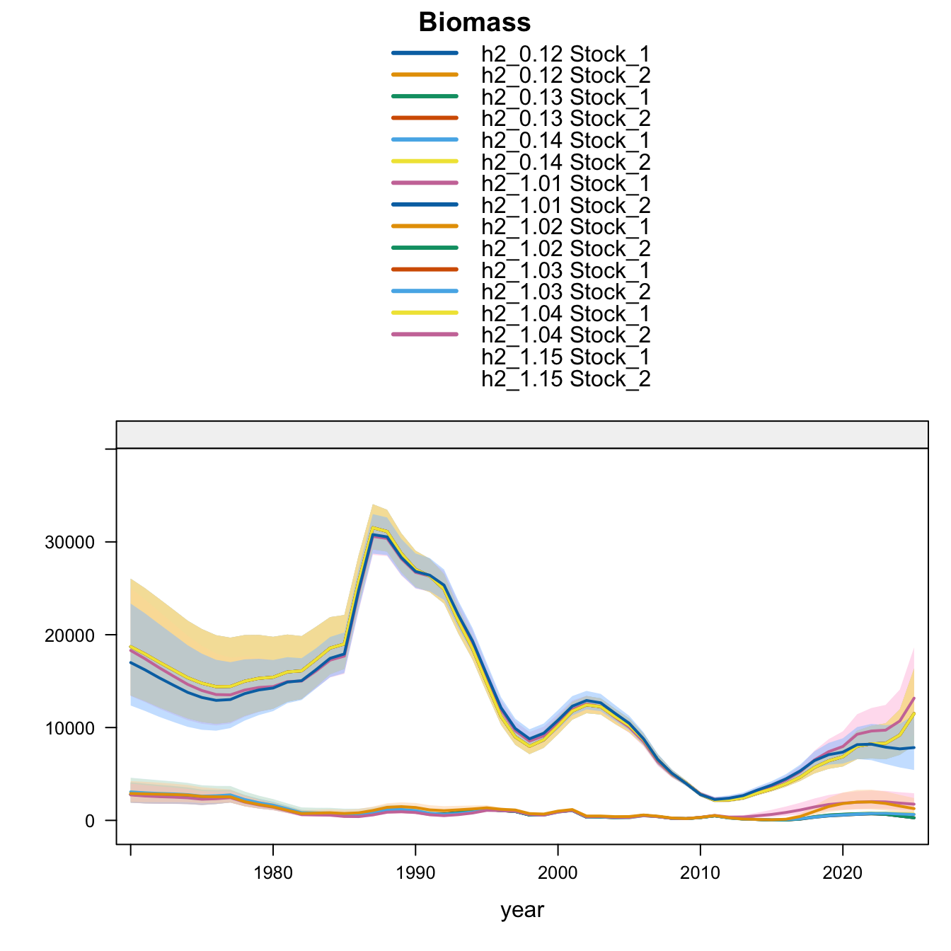
Under the two-stock hypothesis, the updated 0.12, 0.13, and proposed final 0.14 runs have essentially the same southern-stock terminal biomass, recruitment, and fishing mortality. The main differences among those bridge runs are in the FarNorth stock: the 2018 Peruvian CPUE catchability break (0.13) leaves terminal biomass near the very low 0.12 level but sharply reduces terminal fishing mortality. Removing the two Peru acoustic series (1.03) raises FarNorth biomass from the 0.12 level, and adding the same Peruvian CPUE catchability break to that configuration gives proposed final 0.14, which raises FarNorth biomass slightly above 1.03 while cutting terminal fishing mortality further. Adding back the old Peru acoustic series (1.04) produces the largest FarNorth terminal biomass and the lowest terminal fishing mortality among the data sensitivities. The SC13 downweighting sensitivity (SC13_1.15) reduces southern-stock biomass relative to 0.12 while raising FarNorth biomass well above 0.12 but below 1.04.
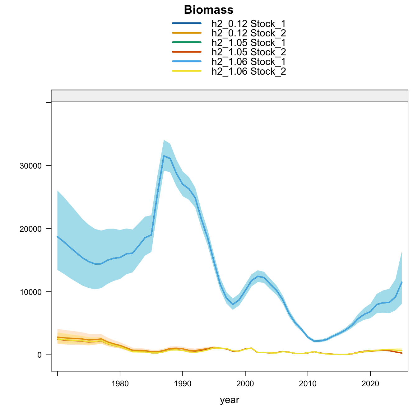
The biomass panel highlights the stock-specific nature of the sensitivity results. Southern-stock biomass is nearly identical for the updated 0.12, 0.13, and proposed final 0.14 bridge runs, lower under SC13_1.15, and higher in the earlier completed 1.02-1.04 trial outputs. The FarNorth biomass trajectory is controlled by the Peru acoustic/CPUE treatment and is much higher in 1.03, proposed final 0.14, 1.04, and SC13_1.15 than in 0.12. The 0.13 catchability-break run stays close to the 0.12 FarNorth biomass trajectory because it keeps the two seasonal Peru acoustic series.
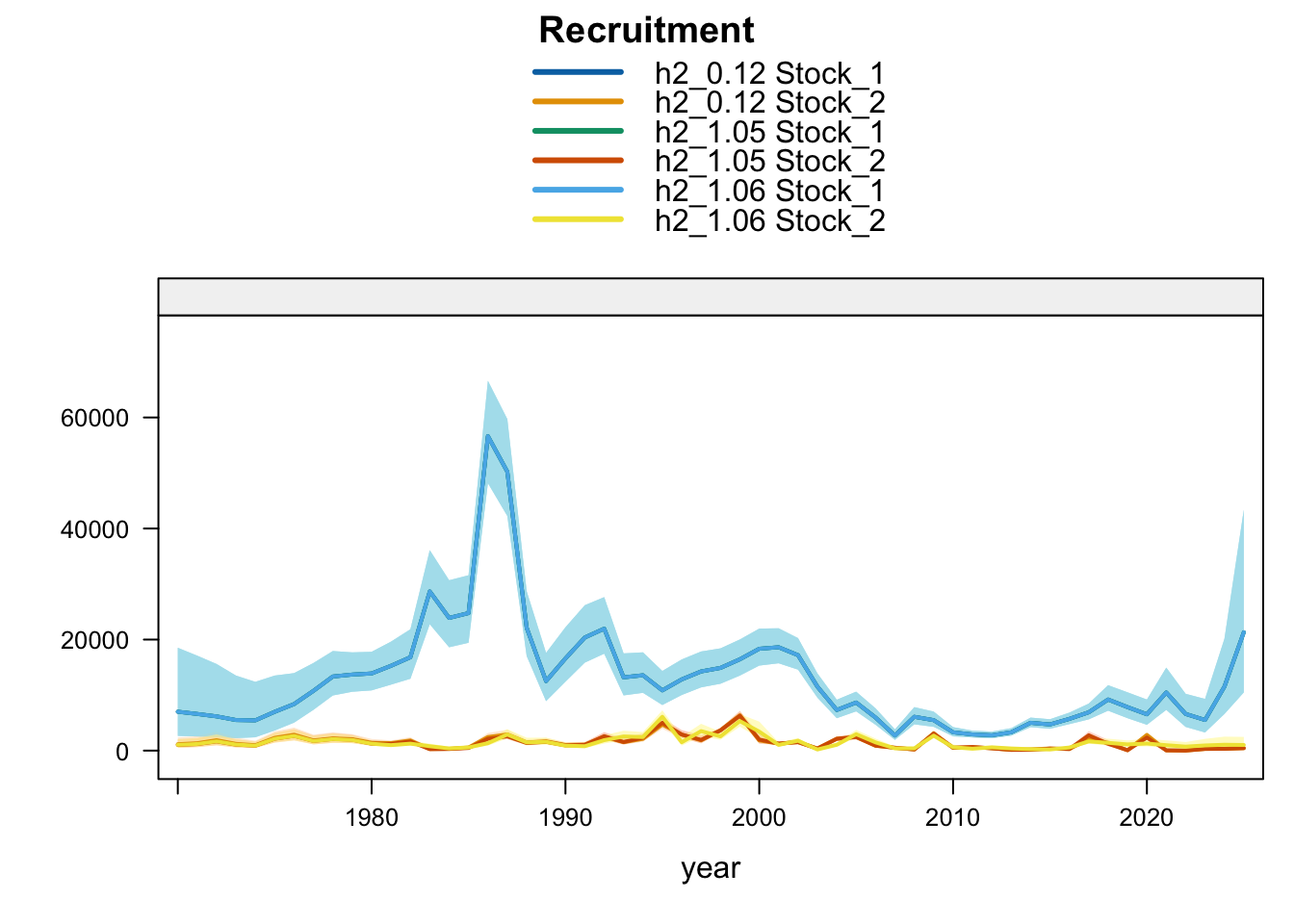
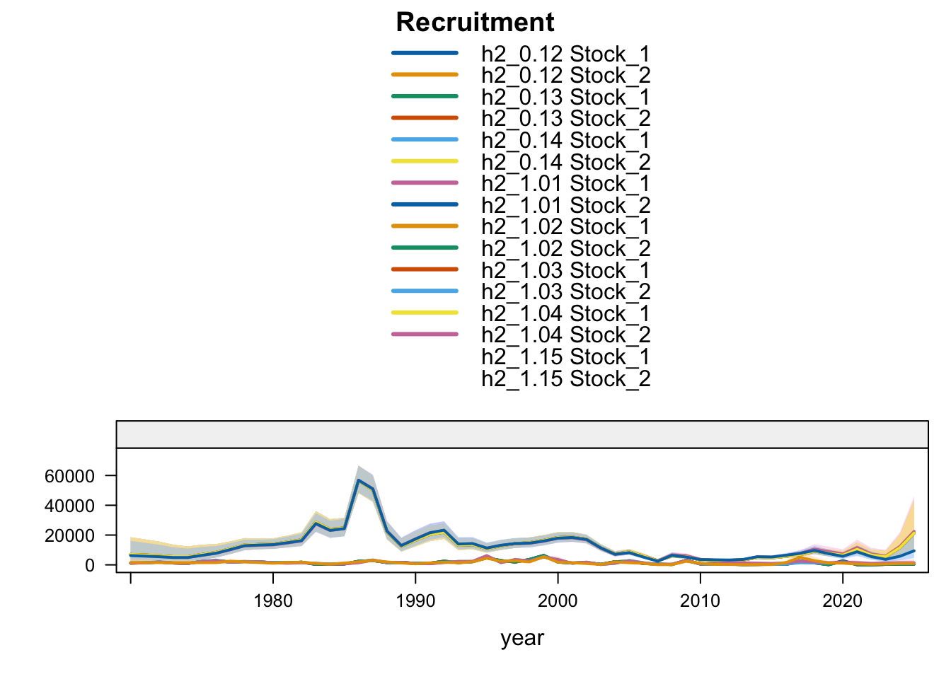
Recruitment follows the same split. Southern-stock recruitment is nearly identical for the updated 0.12, 0.13, and proposed final 0.14 bridge runs, lower under SC13_1.15, and higher in the earlier completed 1.02-1.04 trial outputs. FarNorth recruitment increases when the seasonal Peru acoustic series are removed or replaced, with 1.04 giving the highest FarNorth terminal recruitment among the current data sensitivities. Proposed final 0.14 is slightly above 1.03, while the 0.13 catchability-break run leaves terminal FarNorth recruitment close to 0.12.
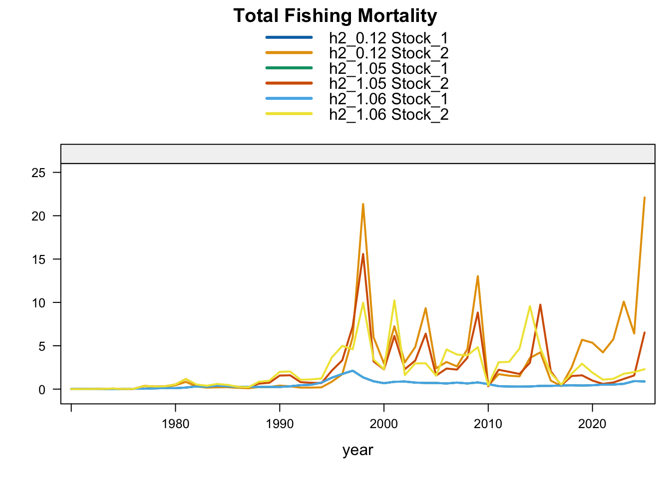
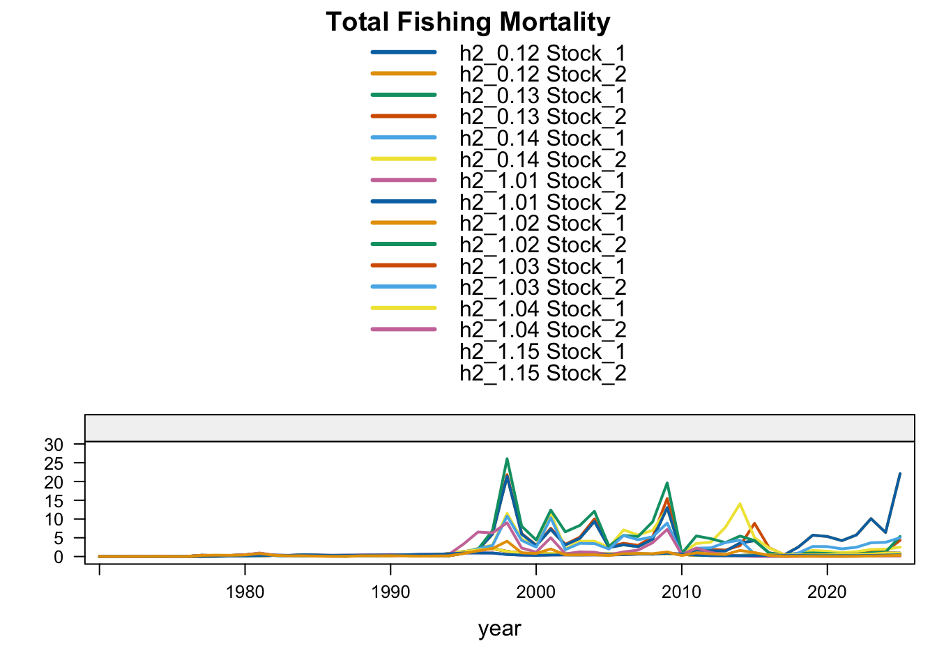
FarNorth fishing mortality is the clearest diagnostic contrast among the two-stock sensitivities. The previous final bridge model (0.12) estimates very high terminal FarNorth fishing mortality, while 0.13, 1.02, 1.03, proposed final 0.14, and especially 1.04 reduce that estimate. The 0.13 result indicates that allowing a 2018 catchability break in the Peruvian CPUE index can reduce the extreme terminal-F estimate even when terminal FarNorth biomass remains close to 0.12. Proposed final 0.14 shows that applying the same break after removing the seasonal Peru acoustic series reduces terminal FarNorth fishing mortality further than 1.03, while keeping the southern-stock fishing mortality close to the updated 0.12 bridge run. SC13_1.15 also moves FarNorth fishing mortality downward relative to 0.12, consistent with fully downweighting the Acoustic N and Peruvian CPUE index series that otherwise pull the FarNorth stock to a very low terminal biomass.
9 Other trials
9.1 Catchability break sensitivity
Model 0.13 is the deterministic sensitivity that starts from the previous final 0.12 bridge configuration and adds a 2018 catchability break for the Peruvian CPUE index. The diagnostics in this section are included to evaluate how that catchability change affects the fitted index scaling, selectivity, and composition residual patterns. No ADNUTS MCMC diagnostics are included for 0.13, and retrospective diagnostics are not shown because the 0.13 retrospective peels have not been run.
9.1.1 Single-Stock Hypothesis
For the single-stock hypothesis, 0.13 changes the way the Peruvian CPUE index is scaled after 2018 while retaining the same underlying data structure as 0.12. The diagnostic emphasis is therefore on whether the catchability break relaxes the recent Peruvian CPUE conflict without creating new residual structure in the retained age- and length-composition data.
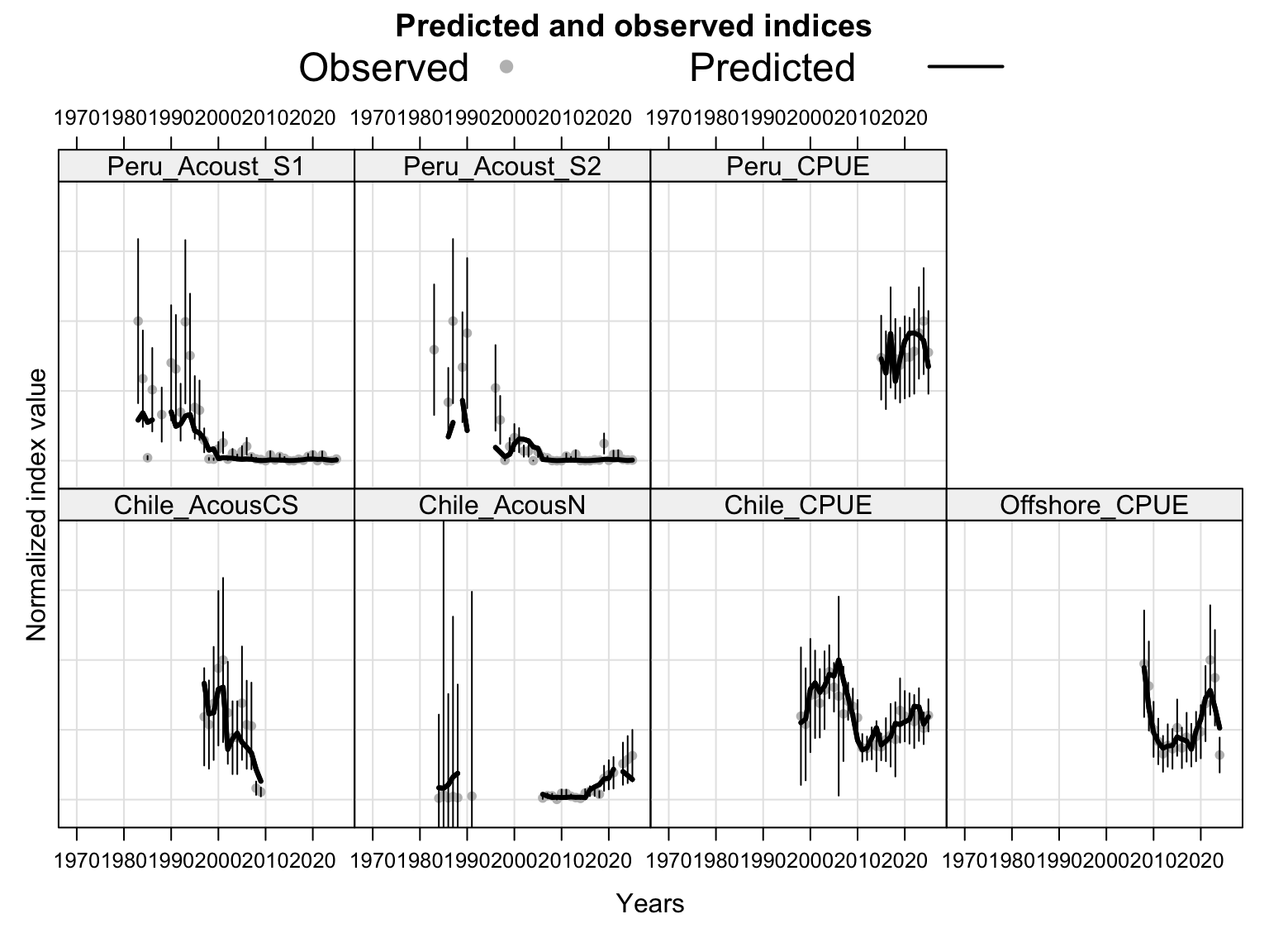
The single-stock index-fit panel checks whether the 2018 catchability break improves the recent Peruvian CPUE fit while preserving the broader fit to the acoustic and other CPUE indices. Because the single-stock model has one aggregate biomass trajectory, any improvement in the Peruvian CPUE fit should be interpreted together with the other retained index series.
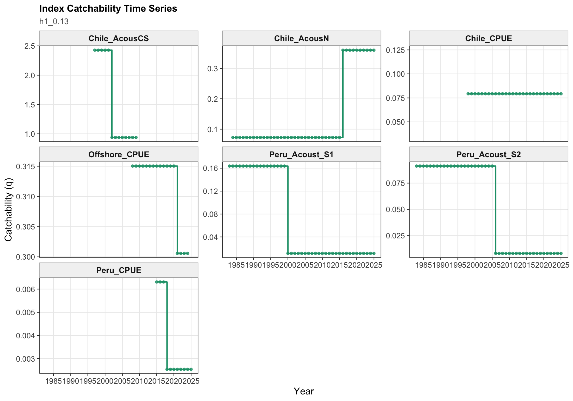
The catchability panel is the primary diagnostic for 0.13. It shows the fitted catchability paths for each abundance index and makes the 2018 Peruvian CPUE break visible as a step change rather than as a change in the observed data.
The selectivity diagnostics provide a check that the 0.13 change is confined to index catchability scaling and does not imply a different interpretation of fishery or survey/index vulnerable biomass through selectivity. The fishery and survey/index panels should therefore be read alongside the catchability panel.
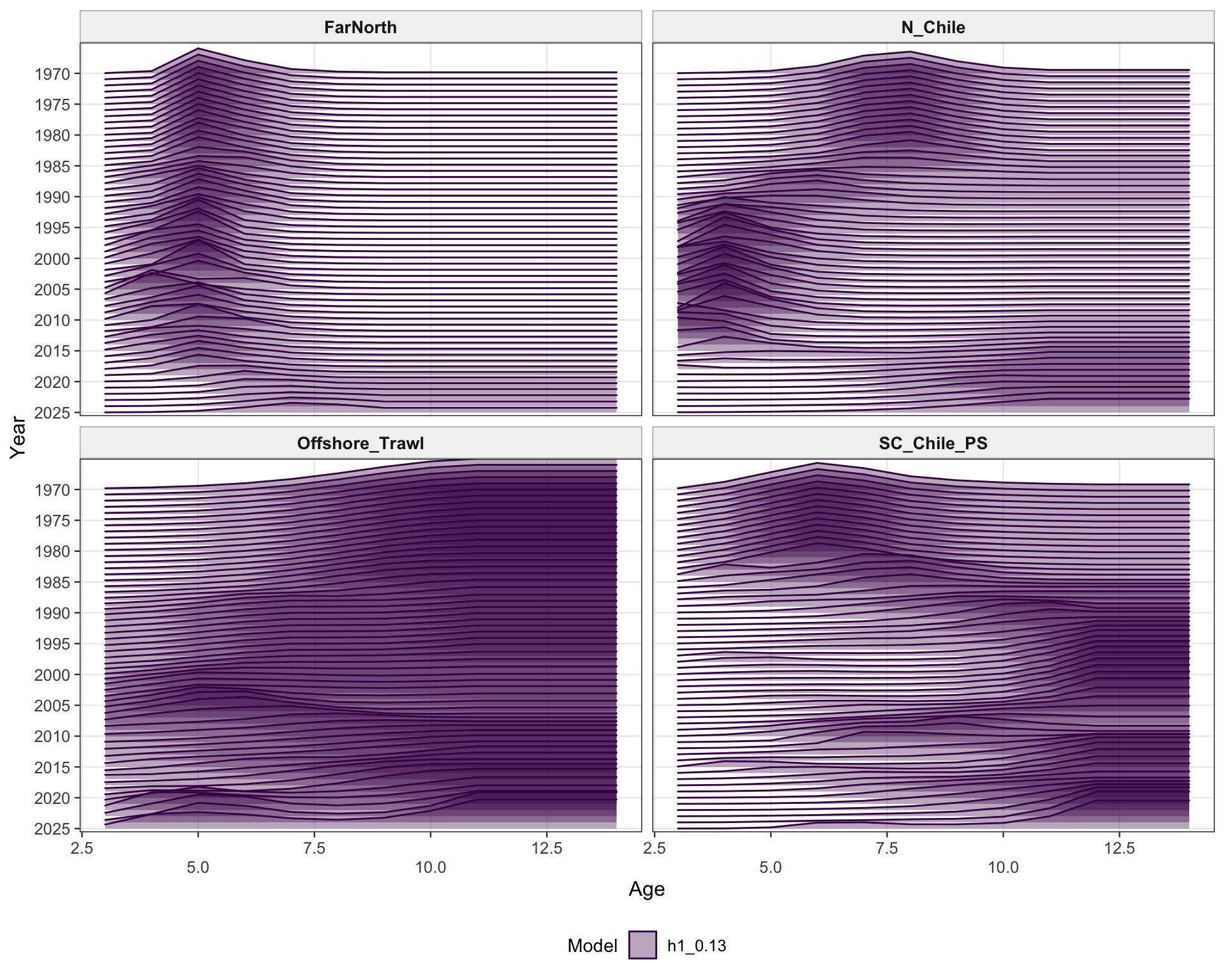
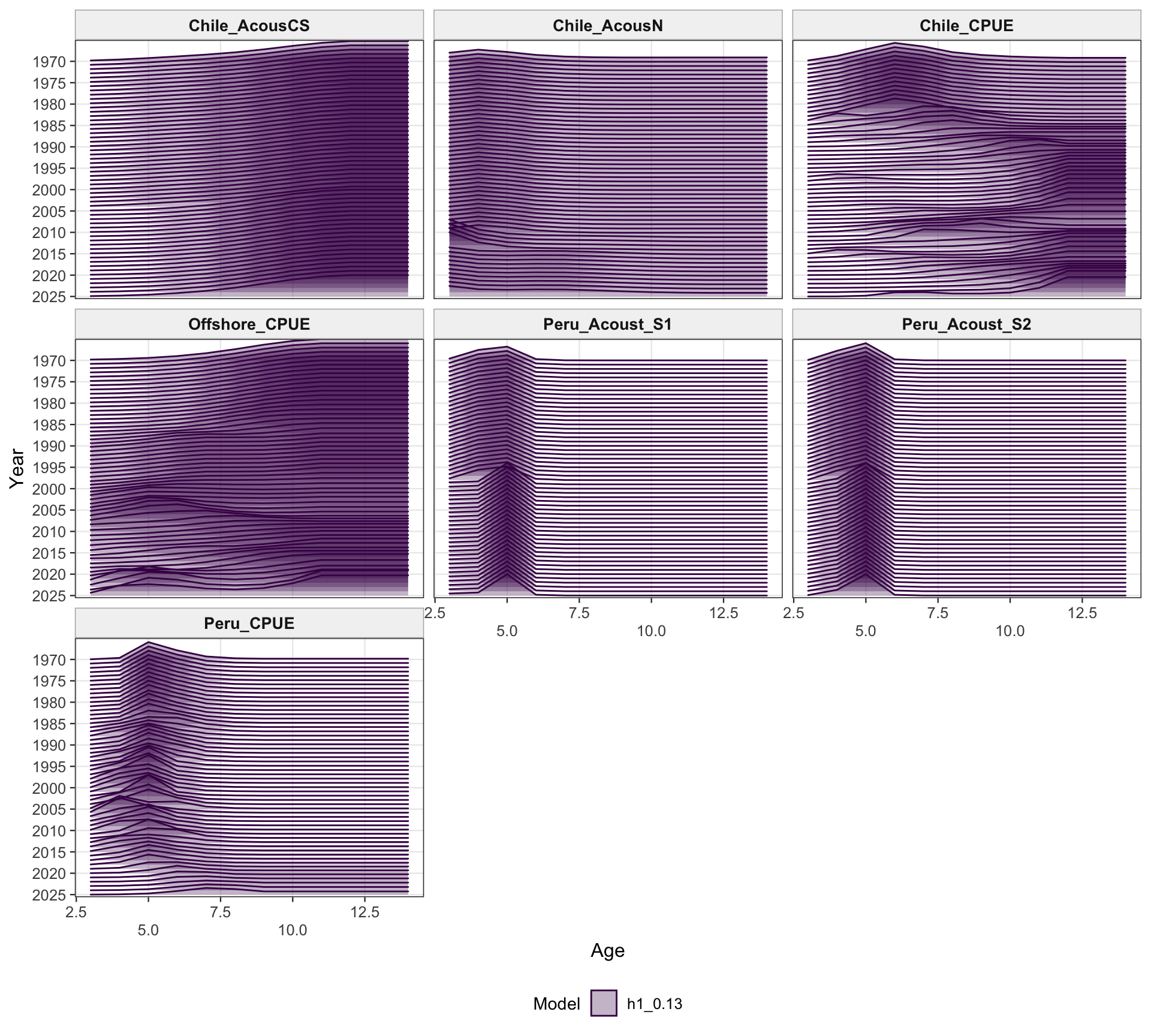
The fishery age-composition diagnostics check whether the 0.13 index-scaling change materially affects the age-fit patterns for the Chilean and offshore-trawl fisheries. These panels should remain broadly comparable with 0.12 because the composition data and selectivity structure are unchanged.
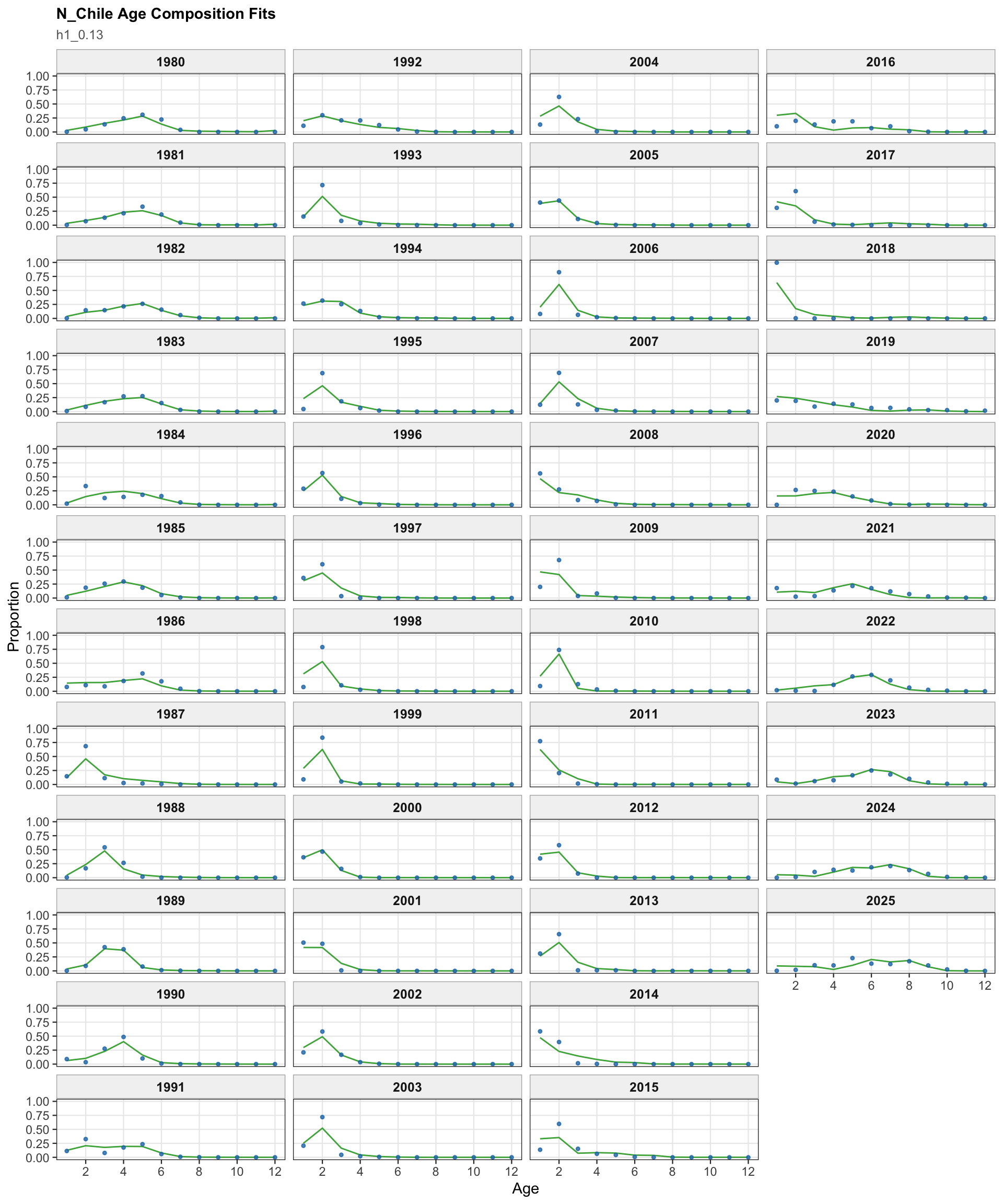
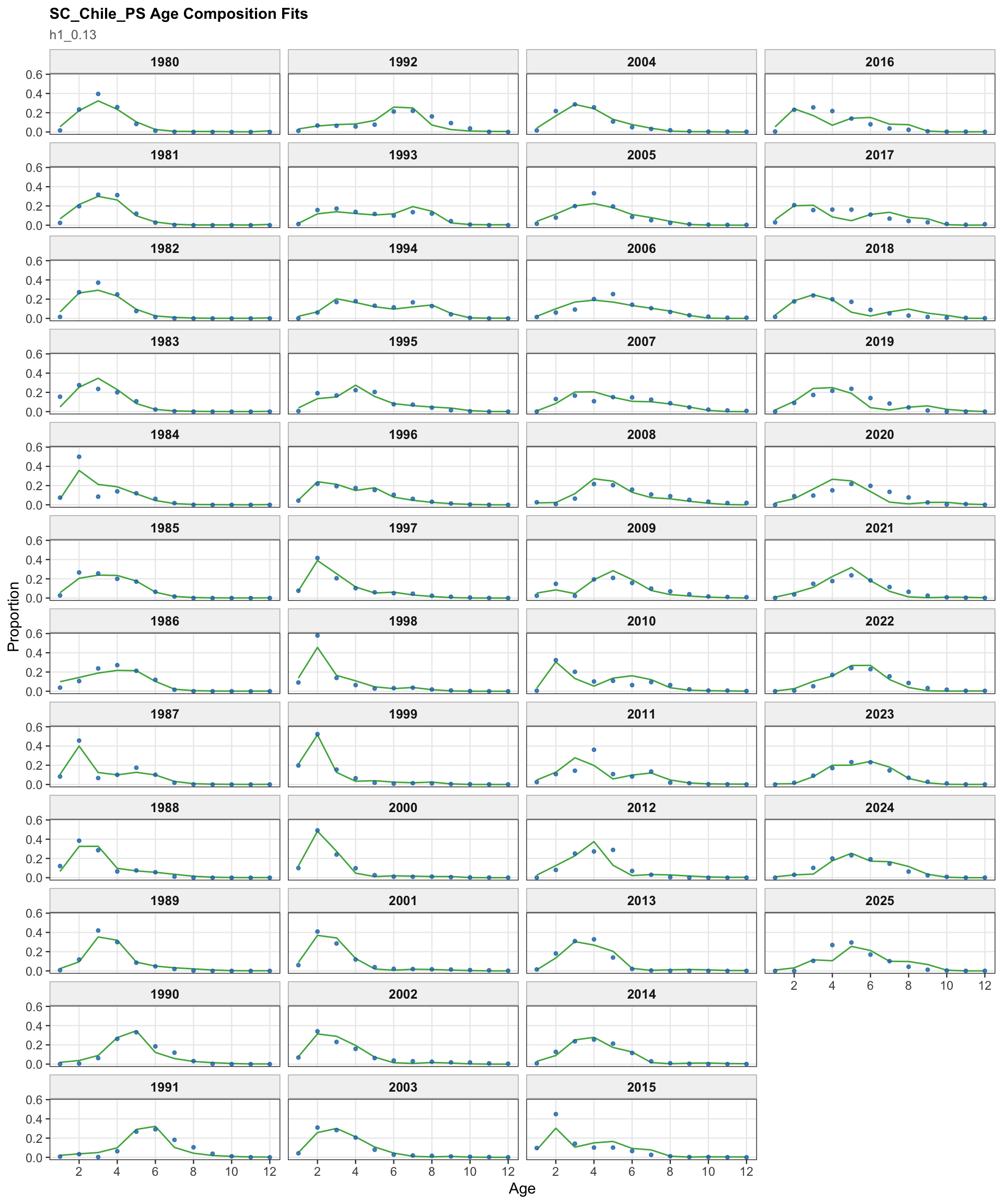
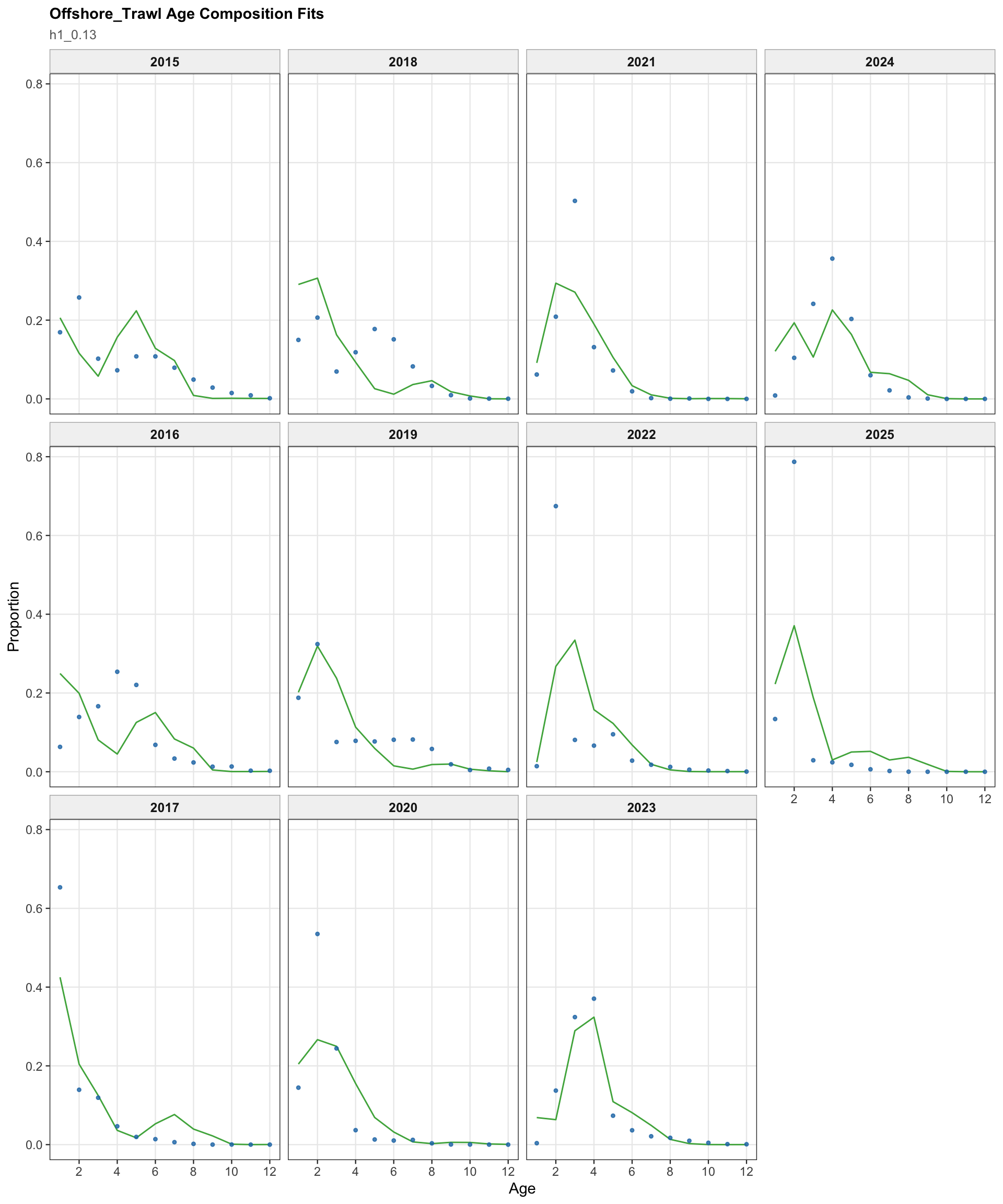
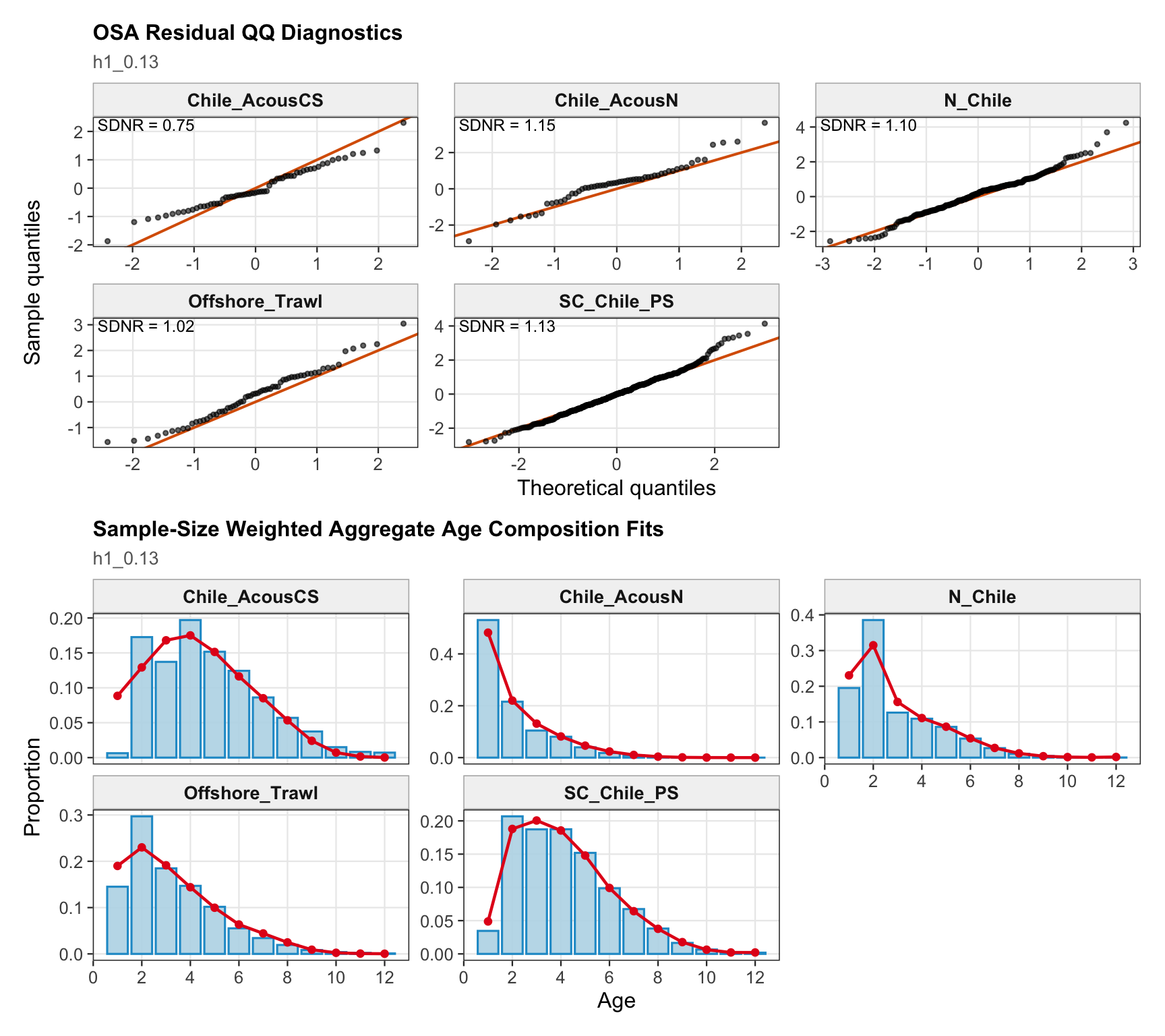
The age OSA and aggregate diagnostics summarize the non-CPUE age-composition residuals for the 0.13 single-stock run. CPUE index age weights are excluded from this diagnostic for the same reason as in the final-model diagnostics: they are not interpreted as age-composition observations here.
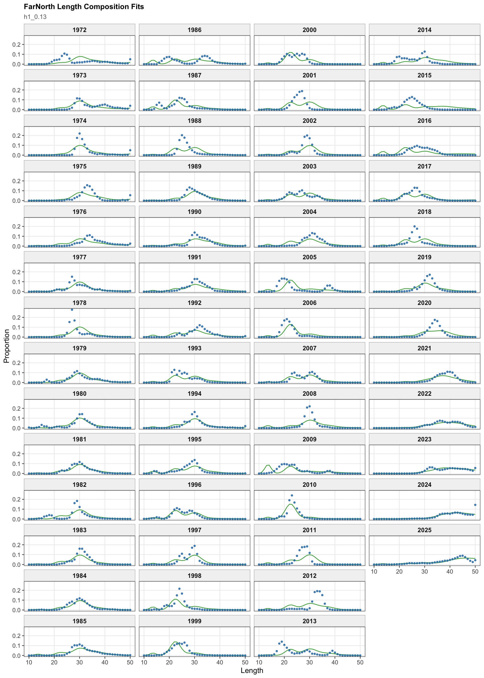
The FarNorth fishery length-composition panels provide the closest composition check on whether the Peruvian CPUE catchability break changes the recent FarNorth signal in a way that conflicts with the fishery length data.
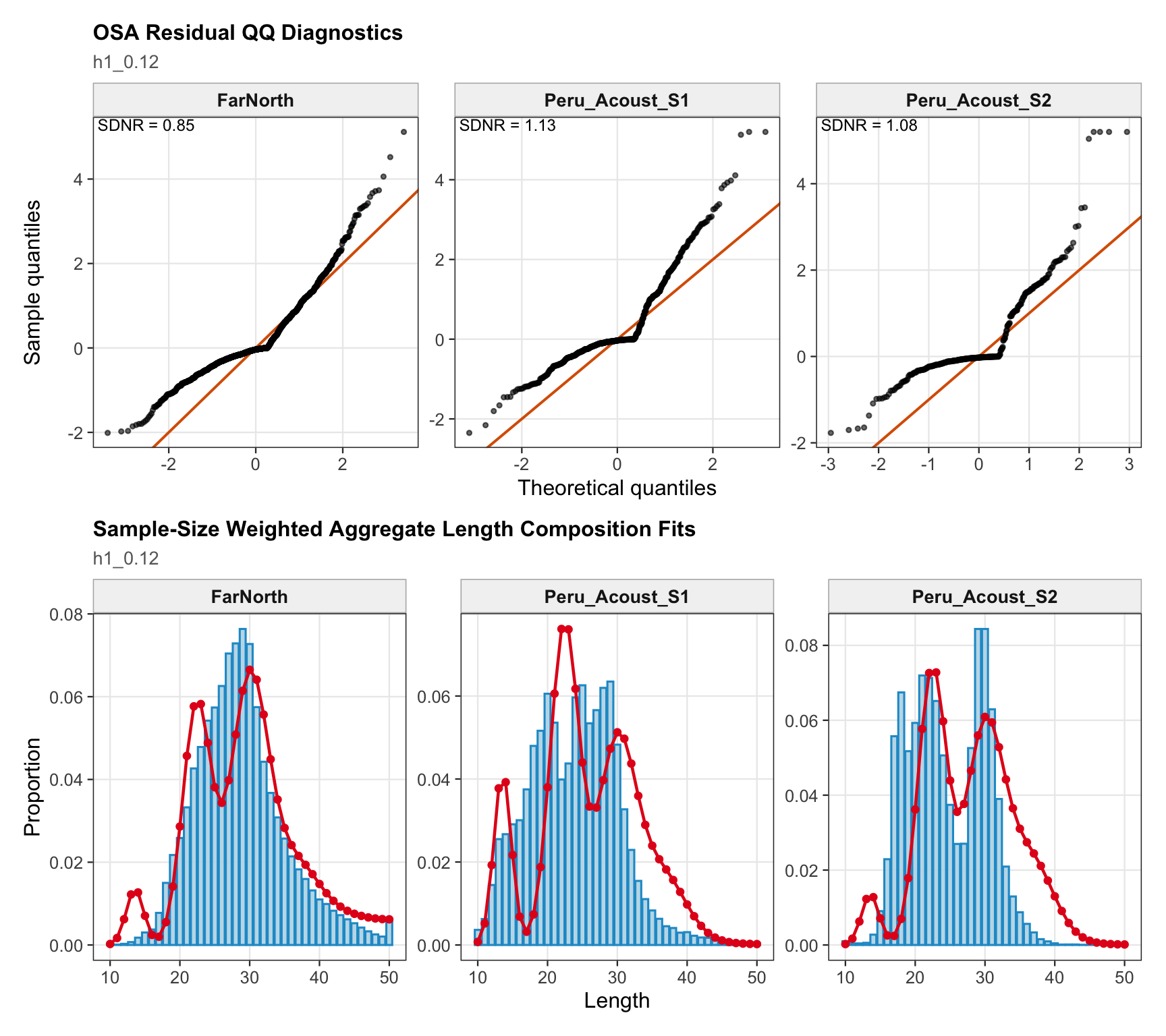
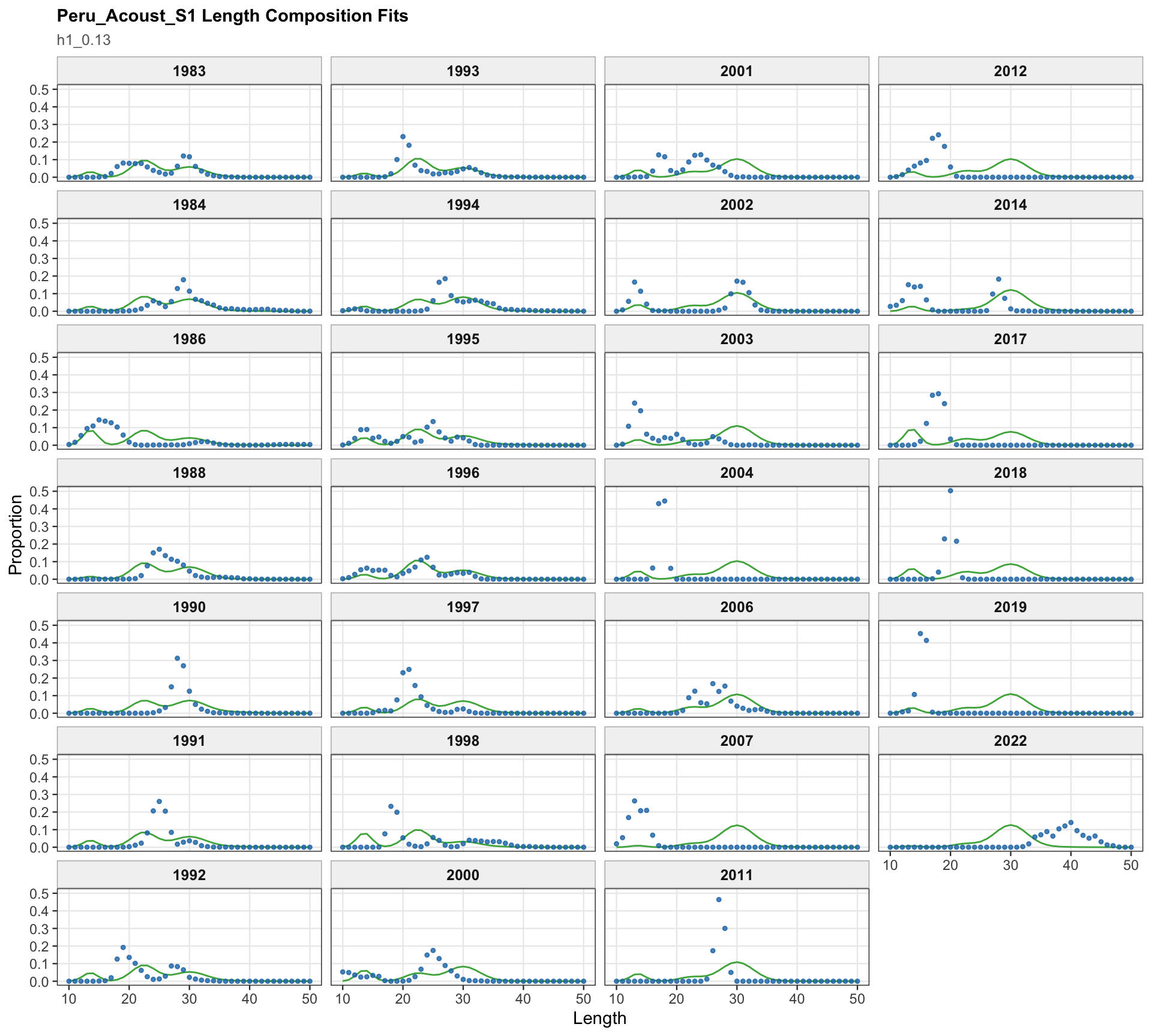
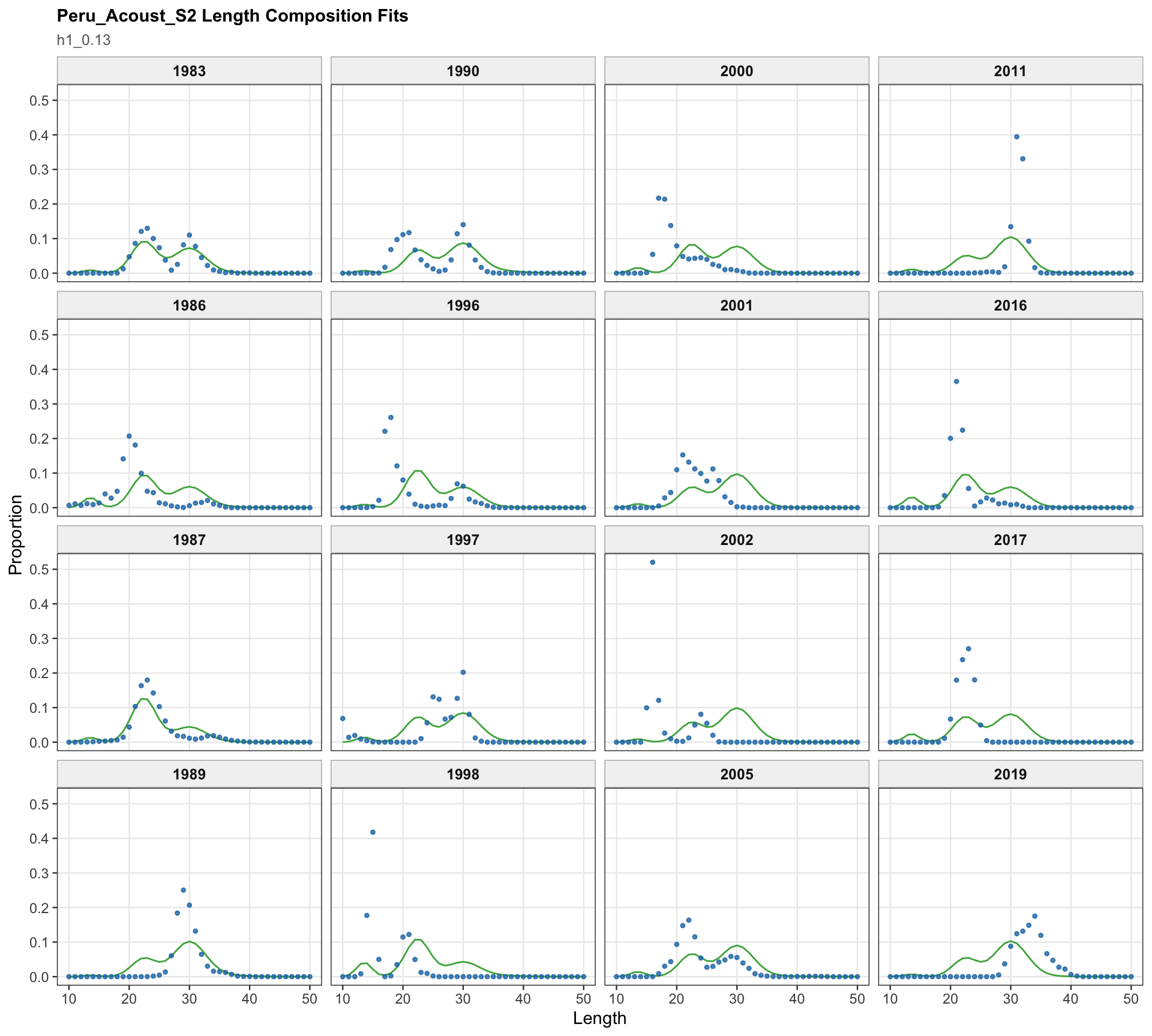
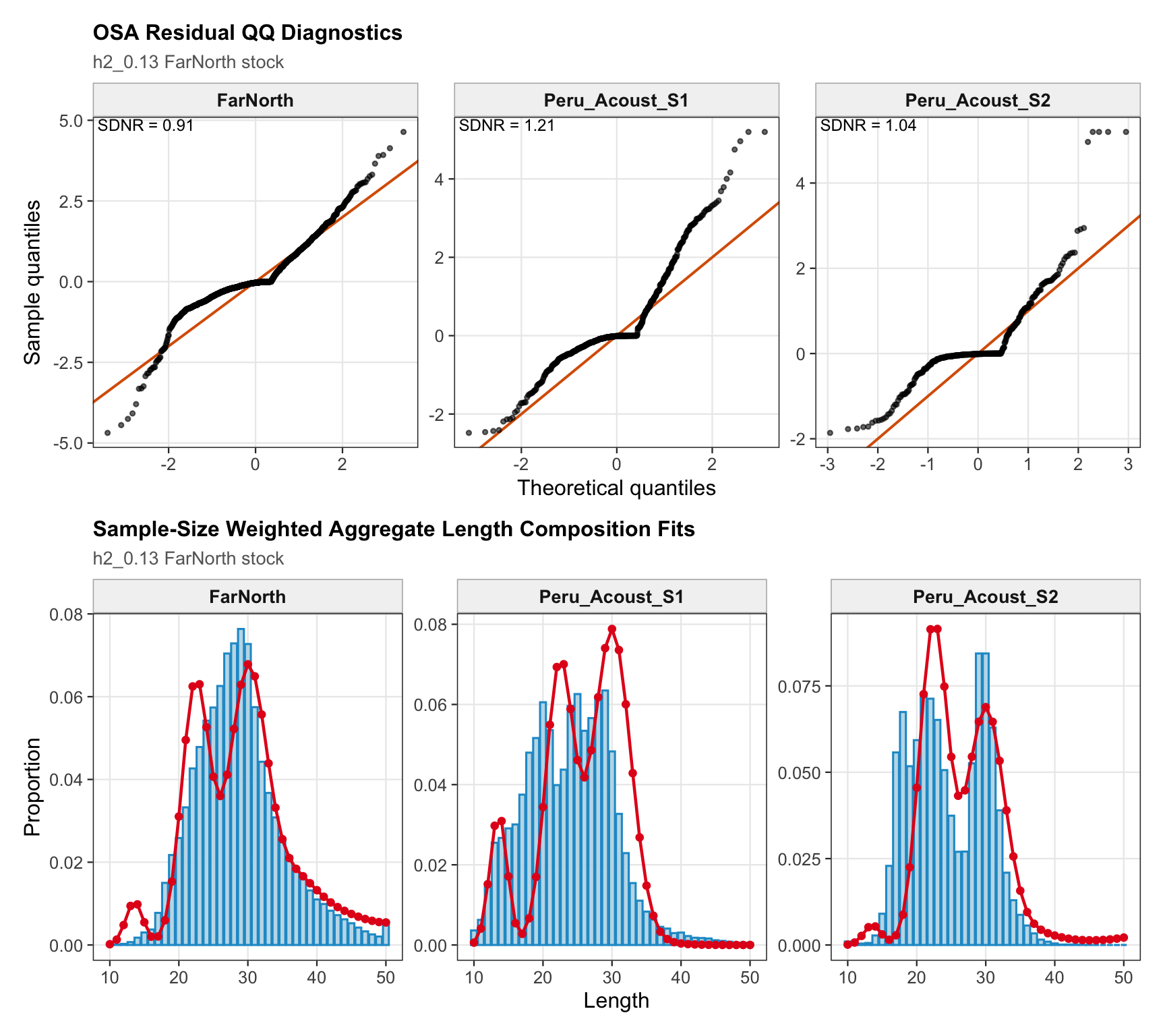
The Peru acoustic length-composition diagnostics are retained for 0.13 because the catchability-break run keeps the two seasonal Peru acoustic series in the model. These panels help separate residual behavior in the Peru acoustic length data from the Peruvian CPUE catchability treatment.
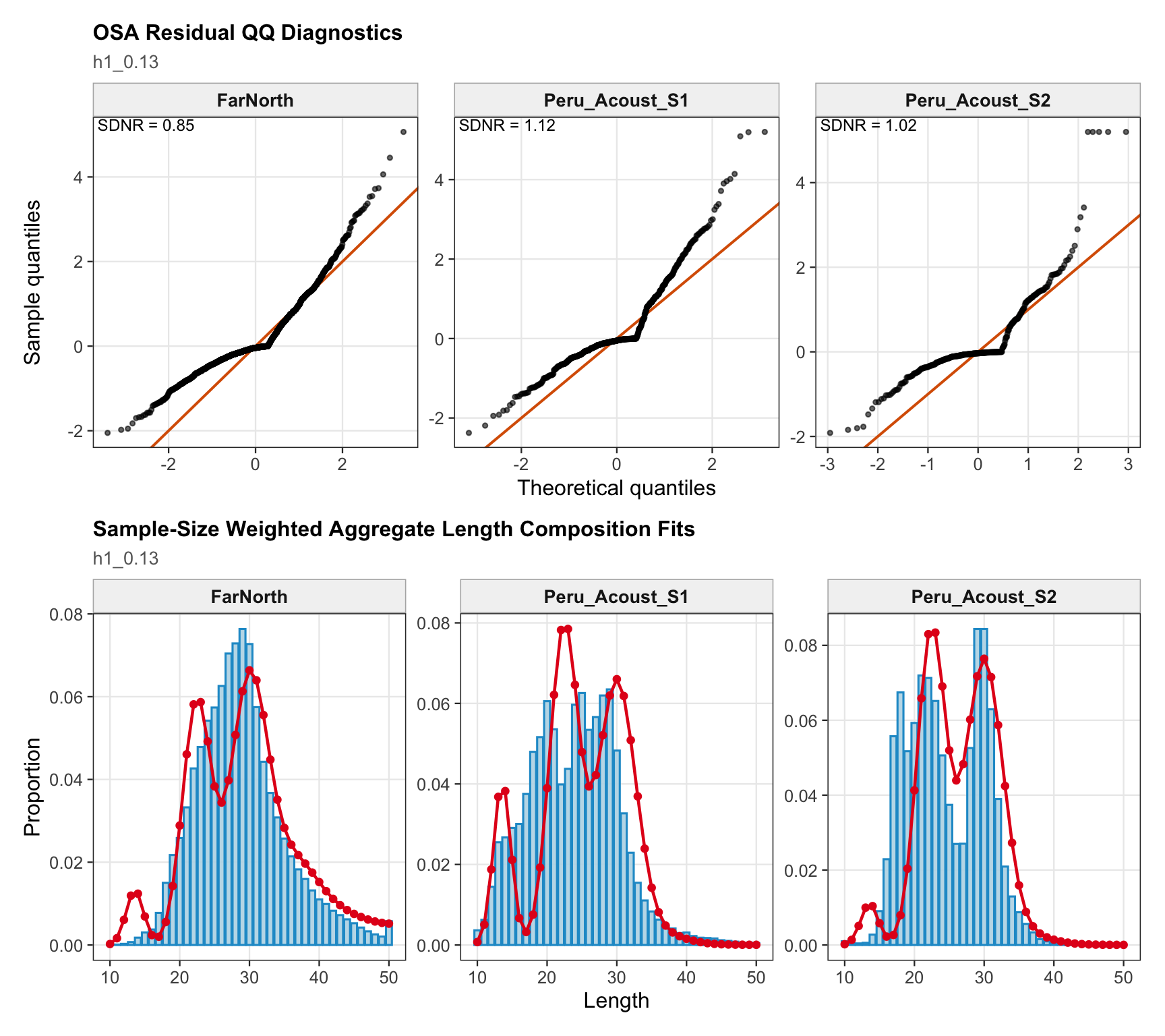
The length-composition OSA and aggregate diagnostics combine the FarNorth fishery and the two seasonal Peru acoustic length series. This provides a compact check on whether the 0.13 catchability treatment leaves the same broad length-residual pattern as the previous final 0.12 run.
9.1.2 Two-Stock Hypothesis
For the two-stock hypothesis, the 0.13 change is most directly relevant to the FarNorth stock because the Peruvian CPUE index informs that component. The diagnostics below therefore emphasize whether the catchability break reduces the extreme recent Peruvian CPUE leverage while keeping the southern-stock diagnostics comparable with the previous final 0.12 configuration.
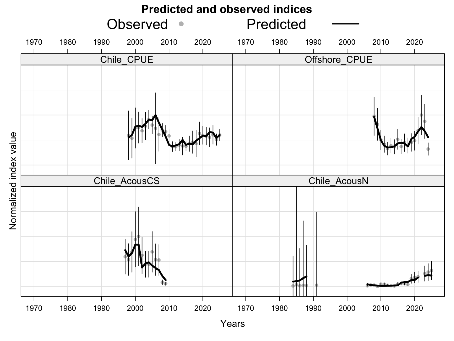
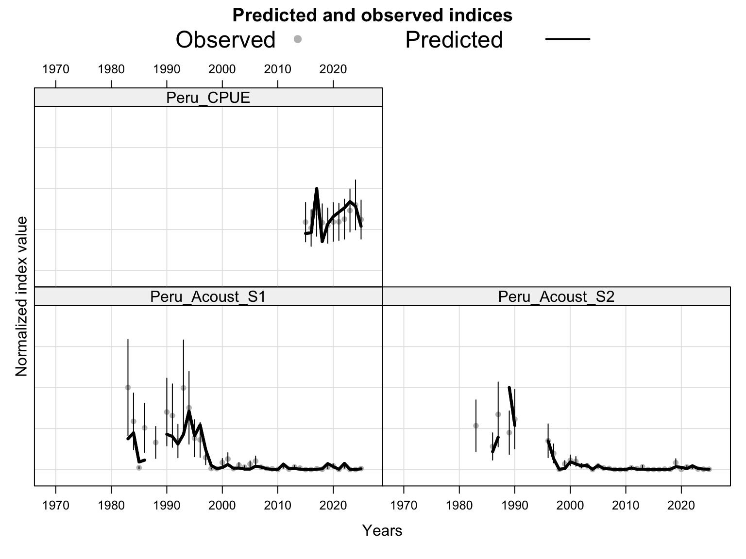
The two-stock index-fit panel shows how the retained abundance indices are partitioned between the southern and FarNorth stocks. The key comparison for 0.13 is whether the Peruvian CPUE index can be fit with a post-2018 catchability shift without requiring the FarNorth biomass trajectory to absorb the full recent index change.
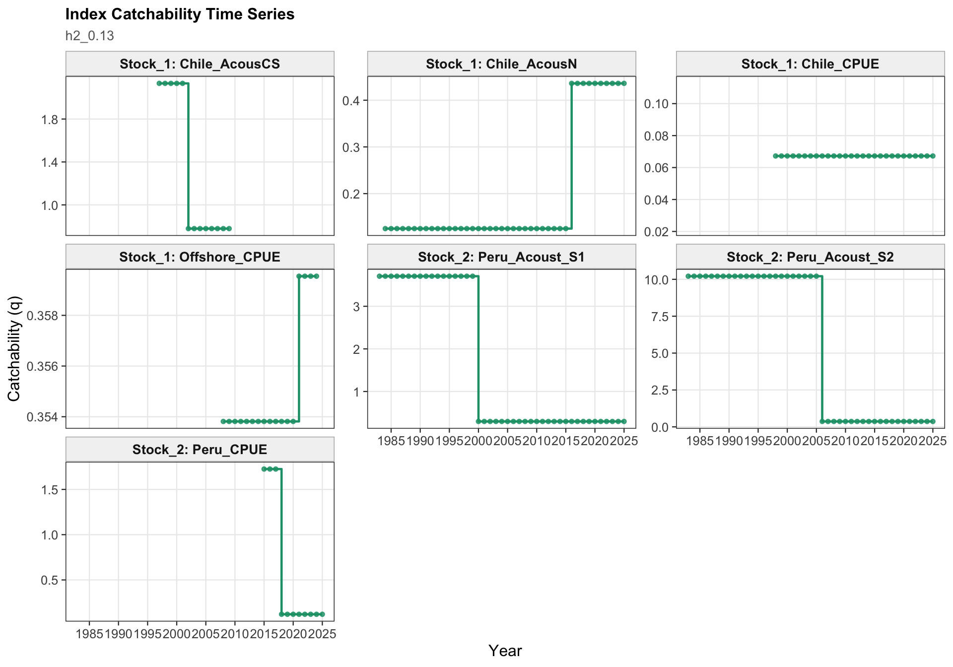
The catchability panel is the central two-stock diagnostic for 0.13. It shows the Peruvian CPUE catchability break in the context of the other retained survey and CPUE catchability paths, including the indices assigned to the FarNorth stock.
The two-stock selectivity diagnostics check whether the southern and FarNorth selectivity patterns remain consistent with the intended 0.13 change. The fishery panel separates the FarNorth fishery from the southern fisheries, while the survey/index panel shows the index selectivity assumptions retained under the catchability-break run.
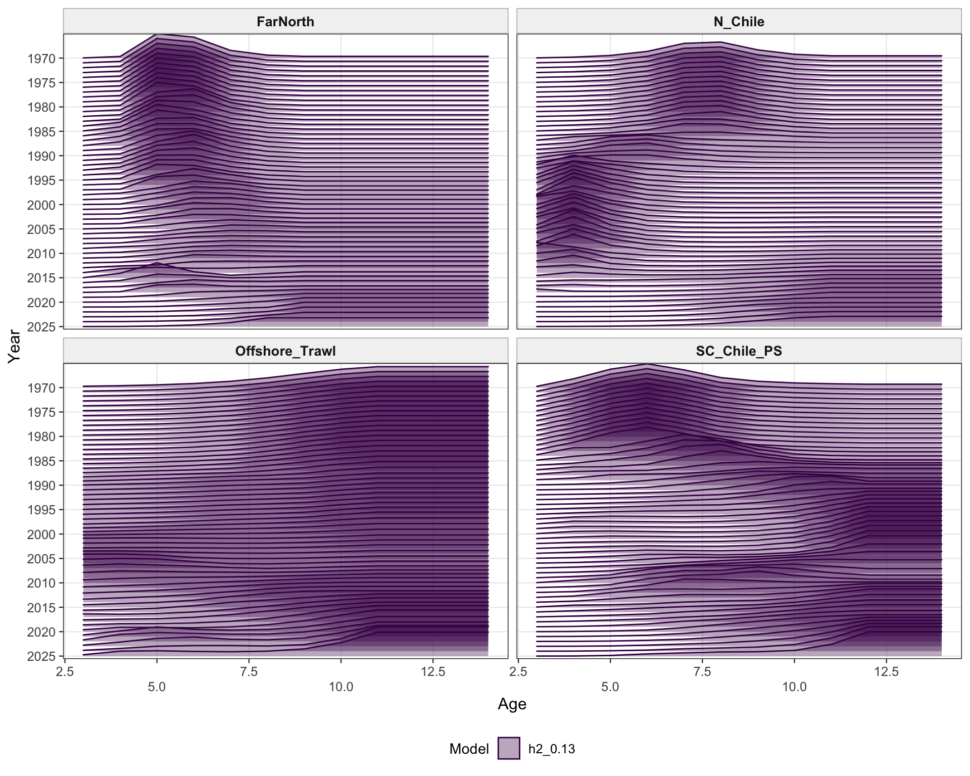
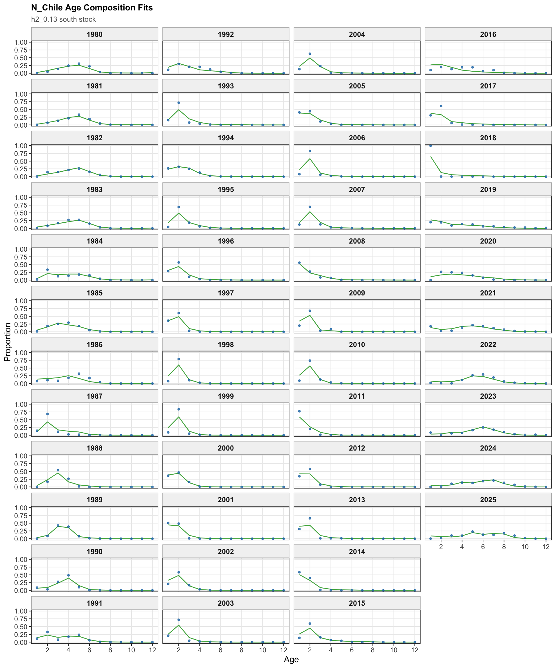
The two-stock age-composition diagnostics are shown for the southern stock. Because the 0.13 change targets the Peruvian CPUE index, these age-composition panels are expected to remain close to the previous final 0.12 southern-stock diagnostics.
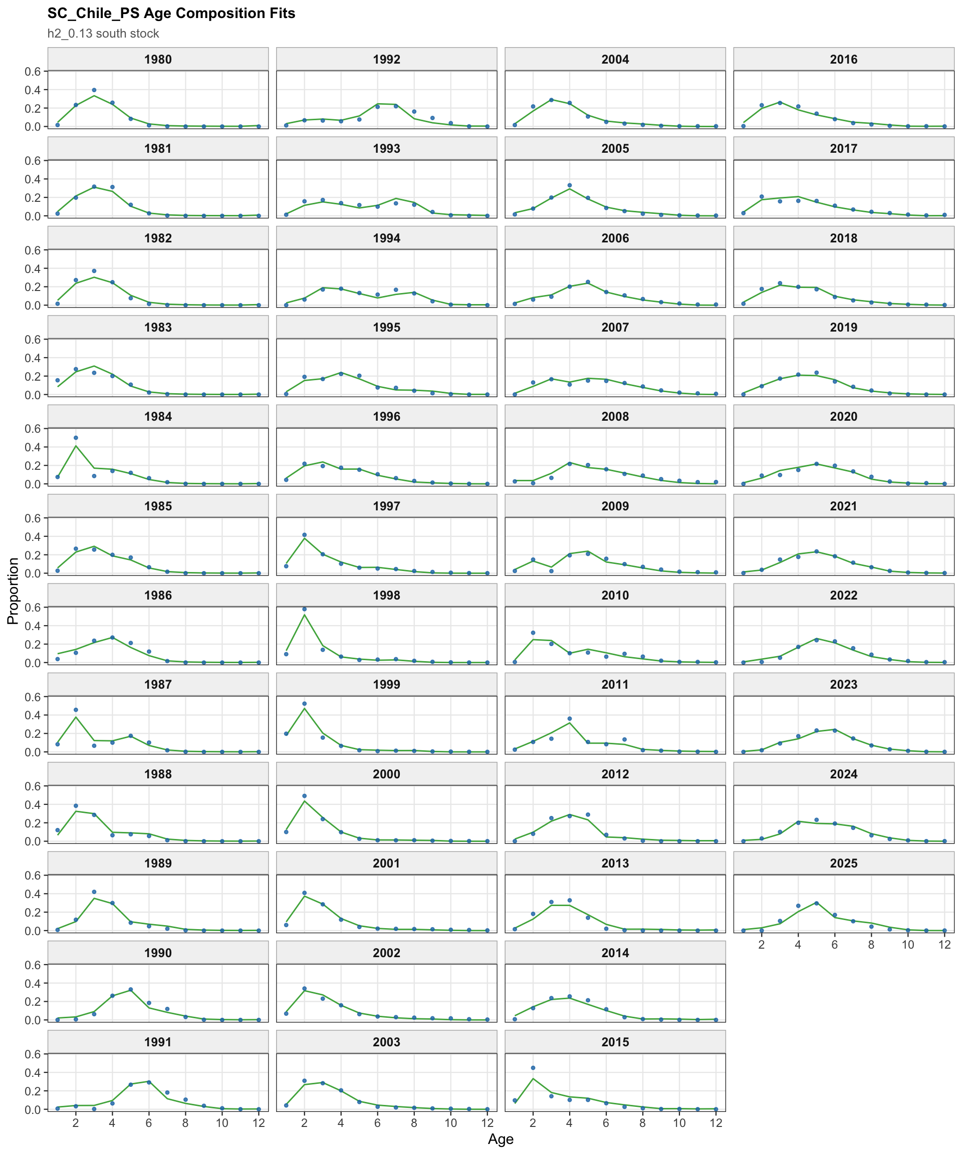
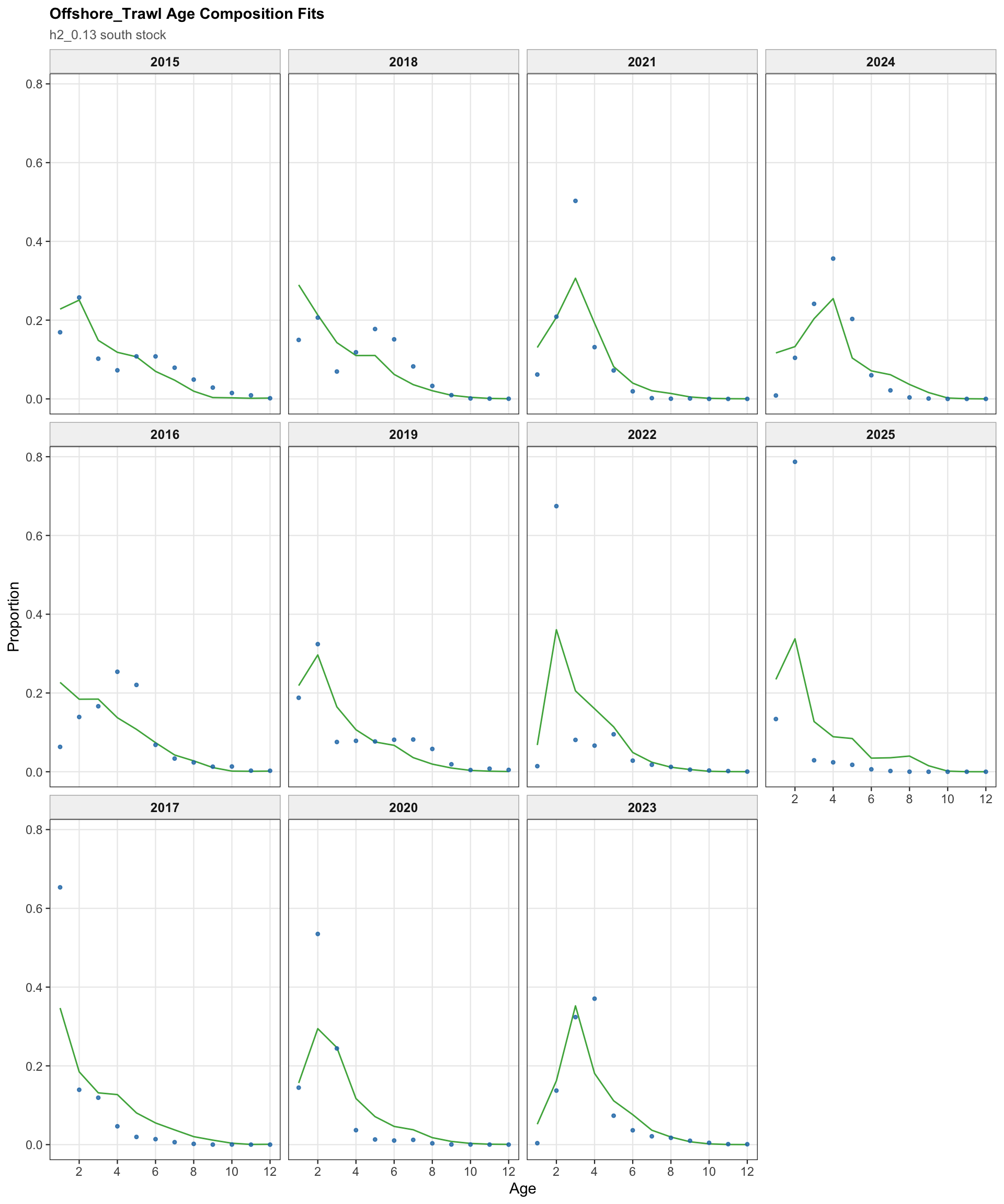
The southern-stock age OSA and aggregate diagnostics summarize the non-CPUE age-composition residuals for 0.13. They provide a check that the FarNorth-oriented catchability change does not introduce a new broad residual pattern in the southern-stock age data.
The FarNorth fishery length-composition diagnostics are central for the two-stock 0.13 run because the Peruvian CPUE catchability break changes the scaling of an index that informs the same FarNorth component as the fishery length data.
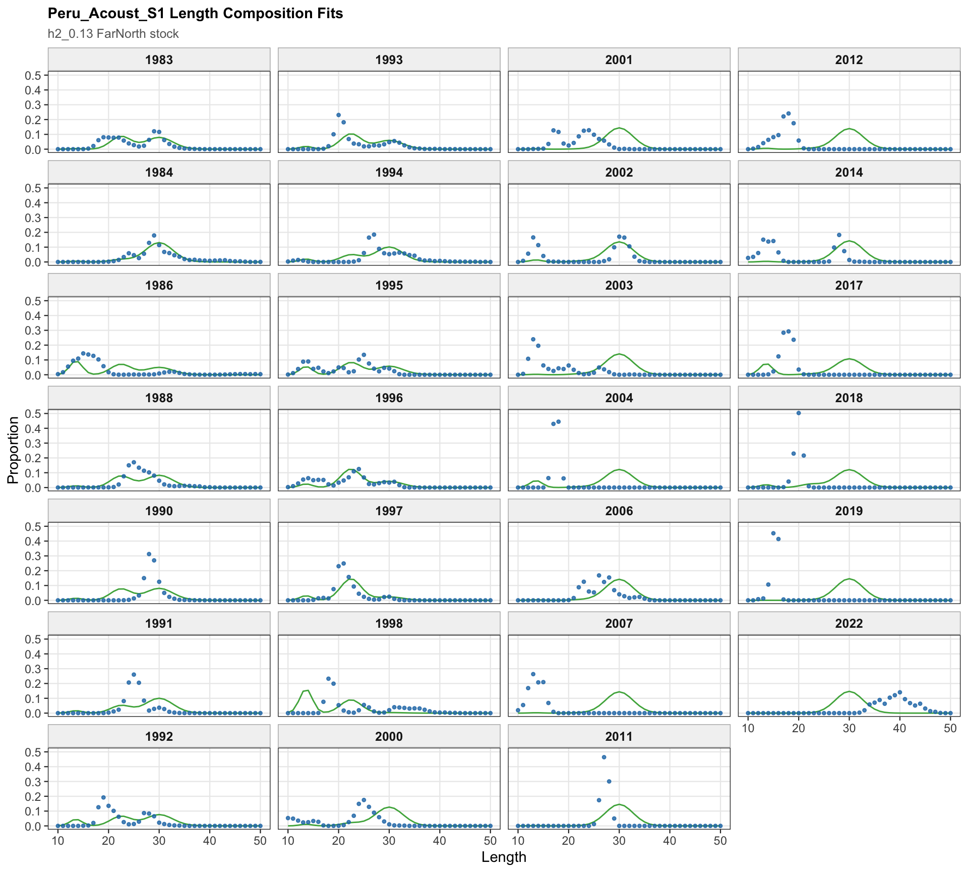
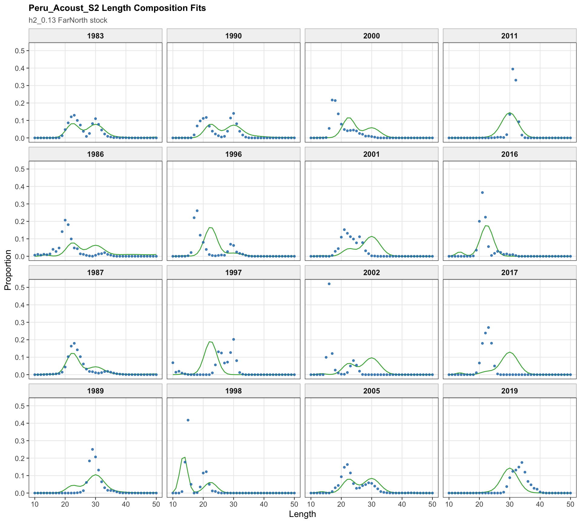
The Peru acoustic length-composition panels remain part of the 0.13 diagnostics because both seasonal Peru acoustic series are retained. These panels help distinguish the Peruvian CPUE catchability signal from any residual structure in the acoustic length observations.
The FarNorth length OSA and aggregate diagnostics combine the FarNorth fishery and the two seasonal Peru acoustic length series. This diagnostic checks whether the catchability break changes the broad length-residual pattern in the FarNorth stock while keeping the same composition sources as 0.12.
These trials are shown separately from the formal data sensitivities because they are diagnostic checks on the Peruvian/FarNorth signal rather than candidate bridge configurations. The motivation is that the Peruvian/FarNorth fishery continues to catch jack mackerel, so the trials ask whether the very low FarNorth biomass and very high terminal fishing mortality in the previous final 0.12 two-stock model are driven primarily by the standardized Peruvian CPUE and seasonal Peru acoustic survey signals.
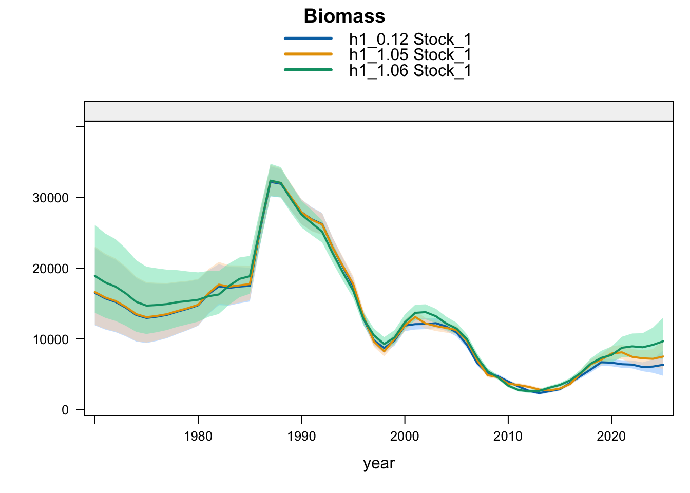
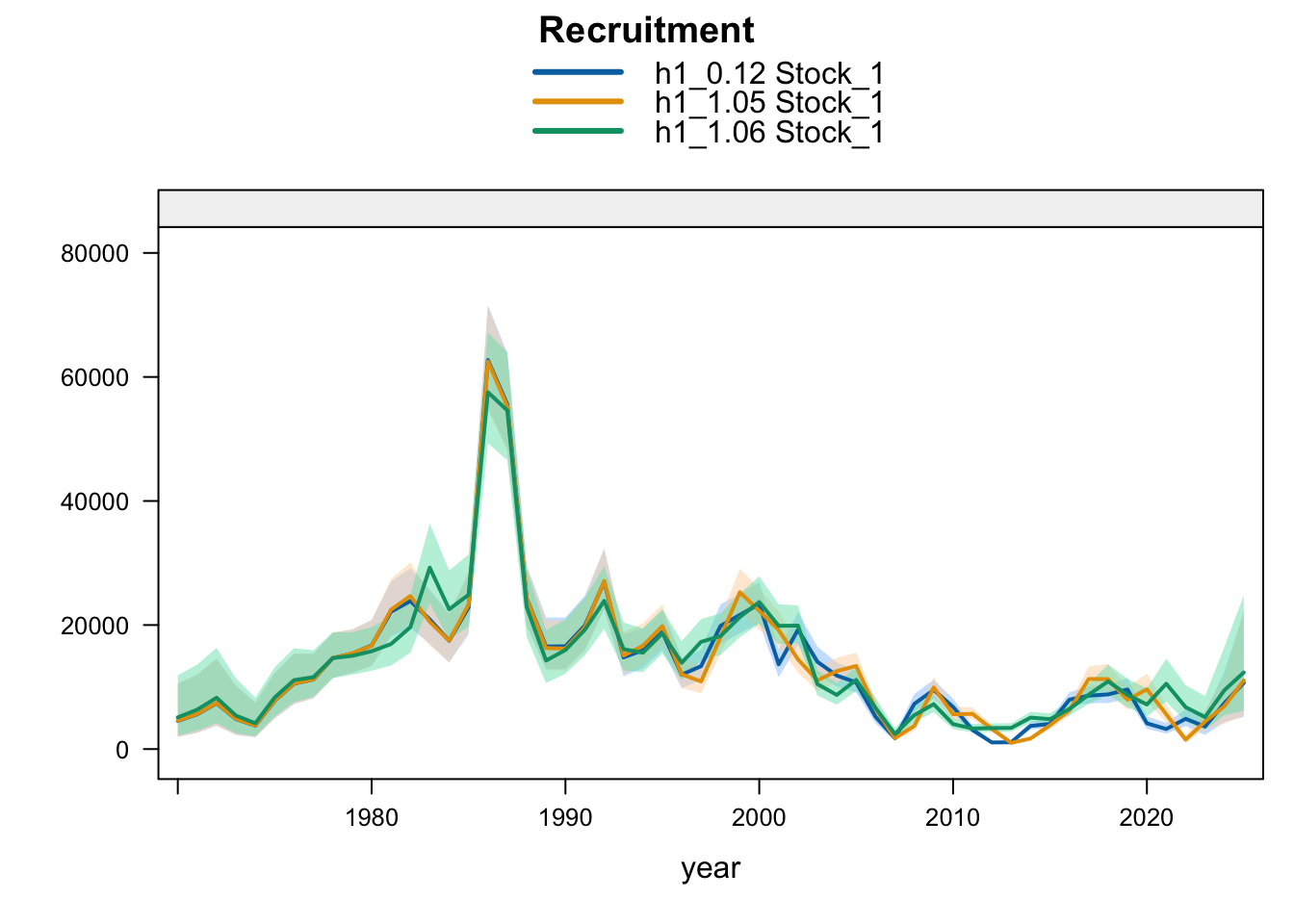
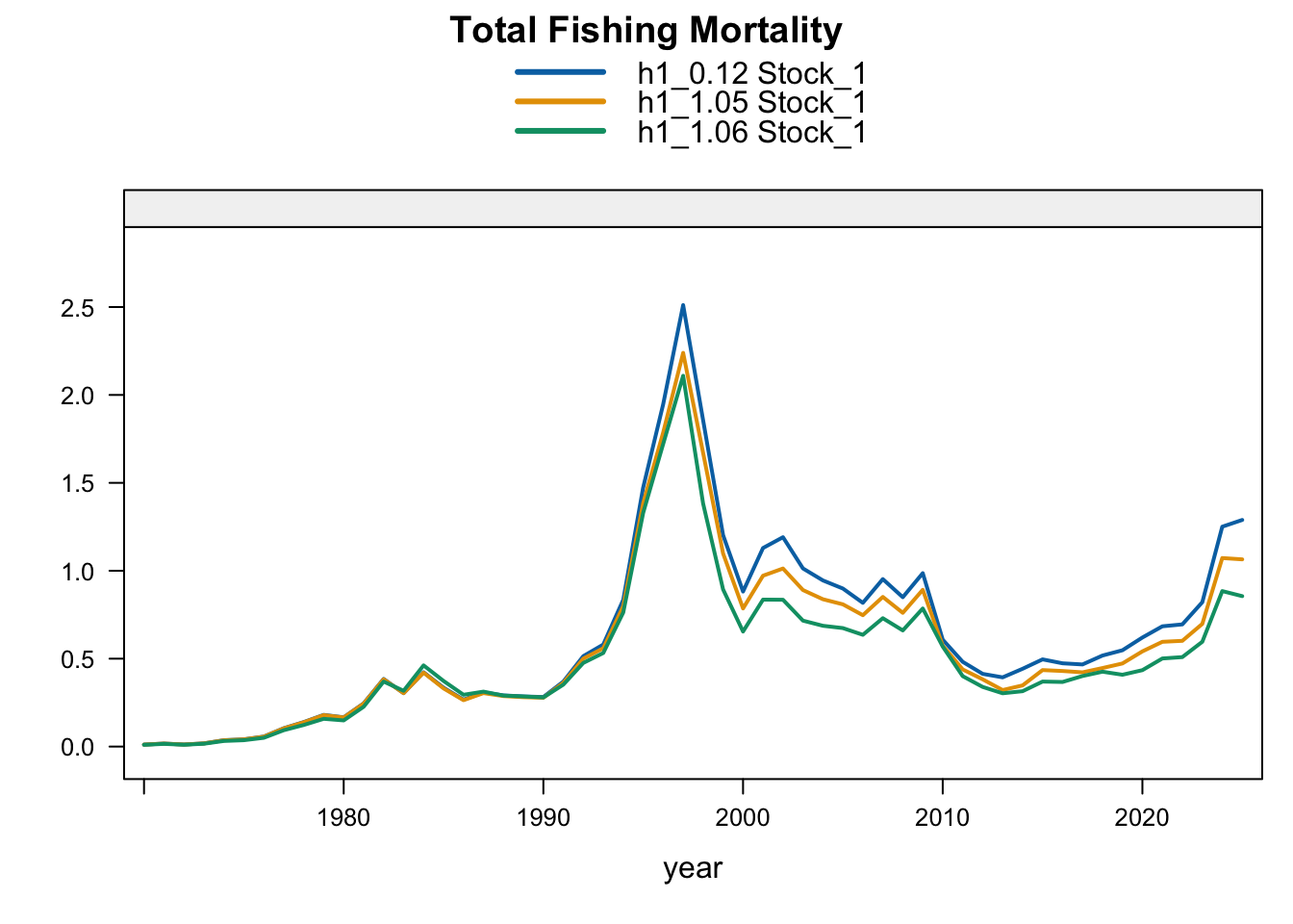
Model 1.05 starts from 0.12 and replaces Peru_CPUE with a noisy (CV = 60%) nominal CPUE series for 1990-2025. Model 1.06 starts from 1.05 and removes the two seasonal Peru acoustic abundance-index series, Peru_Acoust_S1 and Peru_Acoust_S2. Both trials are shown with 0.12 and proposed final 0.14 below, with percent differences calculated relative to proposed final 0.14.
| Hypothesis | Model | Run | N parameters | NLL | Max gradient |
|---|---|---|---|---|---|
| h1 | 0.12 | h1_0.12 | 1871 | 3820.555 | 0.0003189 |
| h1 | 0.14 | h1_0.14 | 1844 | 1301.560 | 0.0003153 |
| h1 | 1.05 | h1_1.05 | 1871 | 3781.912 | 0.0002602 |
| h1 | 1.06 | h1_1.06 | 1843 | 1315.561 | 0.0002240 |
| h2 | 0.12 | h2_0.12 | 1962 | 2641.727 | 0.0001820 |
| h2 | 0.14 | h2_0.14 | 1935 | 1184.311 | 0.0003320 |
| h2 | 1.05 | h2_1.05 | 1932 | 2701.650 | 0.0003403 |
| h2 | 1.06 | h2_1.06 | 1904 | 1270.705 | 0.0002805 |
| Hypothesis | Model | Stock | Year | SSB | Total biomass | Recruitment | Max total F at age |
|---|---|---|---|---|---|---|---|
| h1 | 0.12 | Stock_1 | 2025 | 3211 | 6342 | 10667 | 2.462 |
| h1 | 0.14 | Stock_1 | 2025 | 5773 | 9679 | 12358 | 2.162 |
| h1 | 1.05 | Stock_1 | 2025 | 4097 | 7509 | 11050 | 2.541 |
| h1 | 1.06 | Stock_1 | 2025 | 5768 | 9672 | 12359 | 2.121 |
| h2 | 0.12 | Stock_1 | 2025 | 5398 | 9024 | 11710 | 1.809 |
| h2 | 0.12 | Stock_2 | 2025 | 37 | 277 | 444 | 37.232 |
| h2 | 0.14 | Stock_1 | 2025 | 5398 | 9024 | 11710 | 1.809 |
| h2 | 0.14 | Stock_2 | 2025 | 279 | 669 | 997 | 3.956 |
| h2 | 1.05 | Stock_1 | 2025 | 6719 | 11510 | 21317 | 2.212 |
| h2 | 1.05 | Stock_2 | 2025 | 34 | 274 | 439 | 9.677 |
| h2 | 1.06 | Stock_1 | 2025 | 6719 | 11510 | 21317 | 2.212 |
| h2 | 1.06 | Stock_2 | 2025 | 296 | 693 | 1015 | 3.626 |
| Hypothesis | Model | Stock | Year | SSB (%) | Total biomass (%) | Recruitment (%) | Max total F at age (%) |
|---|---|---|---|---|---|---|---|
| h1 | 0.12 | Stock_1 | 2025 | -44.4 | -34.5 | -13.7 | 13.9 |
| h1 | 0.14 | Stock_1 | 2025 | 0.0 | 0.0 | 0.0 | 0.0 |
| h1 | 1.05 | Stock_1 | 2025 | -29.0 | -22.4 | -10.6 | 17.5 |
| h1 | 1.06 | Stock_1 | 2025 | -0.1 | -0.1 | 0.0 | -1.9 |
| h2 | 0.12 | Stock_1 | 2025 | 0.0 | 0.0 | 0.0 | 0.0 |
| h2 | 0.12 | Stock_2 | 2025 | -86.7 | -58.6 | -55.4 | 841.1 |
| h2 | 0.14 | Stock_1 | 2025 | 0.0 | 0.0 | 0.0 | 0.0 |
| h2 | 0.14 | Stock_2 | 2025 | 0.0 | 0.0 | 0.0 | 0.0 |
| h2 | 1.05 | Stock_1 | 2025 | 24.5 | 27.5 | 82.0 | 22.3 |
| h2 | 1.05 | Stock_2 | 2025 | -87.9 | -59.0 | -56.0 | 144.6 |
| h2 | 1.06 | Stock_1 | 2025 | 24.5 | 27.5 | 82.0 | 22.3 |
| h2 | 1.06 | Stock_2 | 2025 | 6.1 | 3.6 | 1.8 | -8.3 |
9.2 Single-Stock Hypothesis
Under the single-stock hypothesis, replacing the standardized Peruvian CPUE with the noisy nominal CPUE (1.05) increases terminal biomass moderately relative to 0.12 while leaving terminal fishing mortality close to the previous final bridge model. Removing the two seasonal Peru acoustic series as well (1.06) produces a larger biomass increase and lowers terminal fishing mortality below 0.12. Compared with proposed final 0.14, the other trials help separate the effect of a nominal Peruvian CPUE series from the proposed catchability-break treatment.
9.3 Two-Stock Hypothesis
Under the two-stock hypothesis, these trials mainly affect the FarNorth stock and retain a higher southern-stock trajectory from their completed trial configuration. For the FarNorth stock, 1.05 leaves terminal biomass near the 0.12 level but sharply reduces terminal fishing mortality, indicating that the noisy nominal CPUE relaxes the most extreme terminal-F behavior even without removing the seasonal Peru acoustic surveys. Model 1.06 then raises FarNorth terminal biomass and recruitment and further reduces terminal fishing mortality after Peru_Acoust_S1 and Peru_Acoust_S2 are removed, making it a useful comparison with proposed final 0.14.