SAM Diagnostics for the Jack Mackerel Assessment
1 Introduction
1.1 Background and motivation
The Chilean jack mackerel (Trachurus murphyi) stock in the South Pacific is assessed annually by the SPRFMO Scientific Committee using the Joint Jack Mackerel Model (JJM), an age-structured statistical catch-at-age model implemented in AD Model Builder (Fournier et al. 2012). Two competing stock-structure hypotheses are evaluated in parallel: hypothesis H1 (a single shared stock ranging from Peru to the offshore zone) and hypothesis H2 (a separate far-northern stock off Peru combined with a central-southern stock off Chile). The SC13 base model (h1_1.14 and h2_1.14) constitutes the assessment configuration on which the current MSE programme is being conditioned.
1.1.1 The SPRFMO Jack Mackerel MSE programme
A Management Strategy Evaluation (MSE) process for CJM has been underway within SPRFMO for several years and entered a critical delivery phase in 2026. The JM MSE Task Team (TT), chaired by J. Ianelli, is working through a structured programme following the Carruthers et al. (2024) MSE roadmap framework.
A central challenge identified in BM-01 is that the SC13 JJM model is difficult to transfer directly into an MSE Operating Model for four reasons:
- Time-varying selectivity — JJM estimates annual selectivity within blocks, but the block structure and its projection behaviour must be simplified and fixed for OM conditioning;
- Dynamic reference points — JJM’s \(B_\text{MSY}\) and \(F_\text{MSY}\) are re-derived each year and cannot be directly carried into a forward-simulation OM without specifying which biological period they represent;
- Differing fitting and projection assumptions — the estimation model and the projection model in JJM use different assumptions (e.g. about recruitment) that must be reconciled before conditioning;
- Mixed stock-structure differences — H1 and H2 require consistent treatment of the far-northern component to allow meaningful comparison across hypotheses.
BM-01 proposes four simplified alternatives to address these issues: (§6.1) block-based selectivity, (§6.2) a single S–R relationship per hypothesis without regime splitting, (§6.3) fixed static reference points, and (§6.4) harmonised northern treatment across H1 and H2. The TT is scheduled to agree the selectivity block structure and the reference point approach at TT-03 (30 April 2026), with the selectivity question narrowed to at most two candidates at TT-02 (9 April 2026).
For the stock-recruitment relationship (BM-04), the current working prior for H1 is steepness \(h = 0.65\) with recruitment variability \(\sigma_R = 0.6\). An ENSO offshore-drop scenario is also planned as a key robustness test. The OM will be implemented and validated across three platforms — FLR, RTMB, and OpenMSE (DLMtool / MSEtool) — with cross-platform validation addressed in JM-WP-SC14-02.
1.1.2 Role of this SAM analysis
The SAM model is applied here to the H1 configuration as an independent diagnostic tool, not as a replacement for JJM. Its state-space structure and internal data-weighting make it particularly well suited to addressing the open OM-design questions described above — questions that are difficult to resolve from within the JJM framework alone:
- Selectivity (Section 9): SAM’s annual random-walk F provides an objective, statistically grounded basis for choosing how many selectivity blocks are needed and where their boundaries should fall, weighted by the catch volume in each period.
- Productivity and reference points (Section 8): The period-specific Beverton-Holt steepness estimated here can be compared against the working prior \(h = 0.65\) and used to compute block-specific \(F_\text{MSY}\) for the OM.
- Index uncertainty and fleet conflict (Section 6, Section 7): SAM’s internally estimated observation variances and the cross-fleet residual diagnostics identify which of the seven abundance indices carry the most information, which are redundant, and which show systematic trends — directly informing BM-03 (Indices of Abundance: Review and Standardisation) and the choice of MP input data streams for BM-04.
1.2 The State-Space Assessment Model (SAM)
1.2.1 Overview and ICES context
SAM was developed at the Technical University of Denmark and is maintained as an open R package (stockassessment). It has become the standard stock assessment model for the majority of ICES-advised stocks, including North Sea herring, North Sea cod, mackerel, blue whiting, and many others. Although it is not yet widely used outside the North Atlantic, its mathematical foundations are general and apply directly to multi-fleet pelagic assessments such as CJM (Nielsen et al. 2021).
The core idea is to treat the unobserved true population state — numbers-at-age and fishing mortality — as latent random variables that evolve through time according to a process model, while catch and survey observations are linked to those states through an observation model with estimated error variances. This formulation is known as a state-space model and is fitted using the Laplace approximation implemented in the TMB (Template Model Builder) automatic differentiation framework (Kristensen et al. 2016). TMB integrates out the latent states numerically, making the Laplace approximation necessary because the catch equation’s Baranov term renders the model nonlinear in the latent states. The result is a computationally efficient, fully differentiable likelihood that propagates both process and observation uncertainty into all derived quantities.
1.2.2 Population process model
Log-abundance at age follows a random-walk survival equation with process noise:
\[ \log N_{1,t} \sim \mathcal{N}\!\bigl(\mu_R,\,\sigma_R^2\bigr) \qquad\text{(recruitment, treated as a free random effect)} \]
\[ \log N_{a,t} = \log N_{a-1,\,t-1} - Z_{a-1,\,t-1} + \varepsilon_{a,t}, \quad \varepsilon_{a,t} \sim \mathcal{N}(0,\sigma_a^2) \]
The process error \(\varepsilon_{a,t}\) absorbs year-to-year deviations from the deterministic survival equation — deviations that in a classical statistical catch-at-age model would be forced into the residuals of the catch or survey likelihood. This means SAM can fit the data more honestly without over-shrinking recruitment or distorting the F trajectory to compensate for a poor-fitting year.
Fishing mortality also evolves as a latent random walk:
\[ \log F_{a,t} = \log F_{a,t-1} + \eta_{a,t}, \quad \eta_{a,t} \sim \mathcal{N}(0,\sigma_{F,k}^2) \]
Ages that share the same variance parameter \(\sigma_{F,k}^2\) are coupled: they move together through time, effectively defining a selectivity group. The number of F-variance groups, and which ages belong to each group, is a key user choice (see Section 1.5). Fewer groups impose a smoother, more constrained selectivity; more groups allow independent trajectories per age.
1.2.3 Observation model
Catch-at-age observations are log-normal:
\[ \log\hat{C}_{a,t,f} \sim \mathcal{N}\!\bigl(\log C_{a,t,f}^{\text{pred}},\,\sigma_{C,f}^2\bigr) \]
Survey biomass indices (as used here, since the CJM surveys are treated as integrated biomass signals) are:
\[ \log\hat{I}_{s,t} \sim \mathcal{N}\!\bigl(\log(q_s\,\hat{B}_{s,t}),\,\sigma_{I,s}^2\bigr) \]
where \(\hat{B}_{s,t}\) is the model-predicted exploitable biomass for survey \(s\). The observation variances \(\sigma^2\) are estimated from the data, not fixed externally. This is a fundamental difference from JJM, where data weights are set by the analyst. SAM’s internally estimated variances provide a direct, objective measure of the effective weight each data source receives — large variance = low effective weight.
1.2.4 Uncertainty propagation
Because SAM uses the Laplace approximation, the full posterior of all latent states and derived quantities (SSB, \(\bar{F}\), recruitment) is approximated as multivariate normal. This gives analytical confidence intervals for all time-series outputs without requiring MCMC sampling, making it practical to produce annual uncertainty estimates for SSB, F, and recruitment routinely.
1.3 The JJM Model
JJM is a forward-projection statistical catch-at-age model. Numbers-at-age evolve deterministically as:
\[ N_{a,t} = \begin{cases} R_t & a = 1 \\ N_{a-1,\,t-1} \exp\!\bigl(-Z_{a-1,\,t-1}\bigr) & 1 < a < A \\ N_{A-1,\,t-1} \exp\!\bigl(-Z_{A-1,\,t-1}\bigr) + N_{A,\,t-1}\exp\!\bigl(-Z_{A,\,t-1}\bigr) & a = A \end{cases} \]
where \(Z_{a,t} = M_{a,t} + F_{a,t}\). Fishing mortality is decomposed over fleets as:
\[ F_{a,t} = \sum_{f=1}^{F} s_{a,f}\,\Gamma_{f,t} \]
with \(s_{a,f}\) selectivity and \(\Gamma_{f,t}\) the fully-selected fishing mortality. Predicted catch follows the Baranov equation (Hilborn and Walters 1992):
\[ C_{a,t,f} = \frac{s_{a,f}\,\Gamma_{f,t}}{Z_{a,t}}\,N_{a,t} \bigl(1 - \exp(-Z_{a,t})\bigr) \]
Survey indices are modelled as:
\[ I_{s,t} = q_s \sum_a v_{a,s}\,N_{a,t}\,w_{a,t} \]
Observed compositions (age and length) are fitted with a multinomial likelihood. Data weights are specified externally (e.g. Francis reweighting, Francis (2011)).
1.4 Key differences between JJM and SAM
| Feature | JJM | SAM |
|---|---|---|
| Framework | Deterministic forward projection (ADMB) | State-space model with Laplace approximation (TMB) |
| Process error | None — \(N\) fully determined by catch | Random walk in \(\log N\) and \(\log F\) |
| Composition data | Age and length proportions (multinomial) | Age proportions only (log-normal) |
| Data weighting | External (Francis, input ESS) | Internal — \(\sigma^2\) estimated |
| Selectivity | Constant within user-defined year blocks | Annual random walk; blocks optional |
| Catchability | Fixed \(q\) per survey | Fixed \(q\); residual trends reveal drift |
| Reference points | Computed internally per selectivity block via SPR/YPR | Externally estimated |
| Uncertainty | Hessian-based delta method | Laplace approximation; MCMC optional |
1.5 SAM in the MSE context
The MSE process for CJM requires an Operating Model (OM) that can generate plausible stock trajectories under different harvest control rules. The OM is typically conditioned on the assessment model: its parameter estimates, uncertainty structure, and dynamic assumptions are inherited directly from the assessment. Three open questions are particularly important for the OM design, and SAM provides evidence for each.
1.5.1 1. Selectivity: constant blocks versus annual random walk
JJM parameterises selectivity as constant within user-defined year blocks. The OM inherits these blocks directly, meaning the OM’s F trajectory in the projection period is governed by the selectivity pattern of the most recent block. If that block does not accurately represent the current fleet behaviour — because it is too long, or because the true selectivity has been gradually shifting — the OM will be biased.
SAM estimates selectivity annually via a random walk and therefore reveals when the selectivity shape changed significantly. The block analysis in Section 9 translates those SAM-estimated change points into suggested block boundaries for JJM, ranked by importance. The OM designer can then choose the minimum number of blocks that captures the dominant selectivity regimes without overfitting.
The key trade-off is:
- Too few blocks: selectivity is over-smoothed; the OM misrepresents the current fleet’s age targeting and will generate biased F projections.
- Too many blocks: each block is estimated from fewer data, increasing uncertainty in selectivity; the OM carries more estimation noise into projections.
1.5.2 2. Biological reference points: fixed versus time-varying
JJM already computes biological reference points (\(F_\text{MSY}\), \(B_\text{MSY}\), \(B_{40\%}\)) internally via equilibrium per-recruit (SPR/YPR) analysis within each selectivity block. Because JJM estimates a separate selectivity pattern for each block, the reference points it reports are inherently block-specific: changing the selectivity block structure directly changes the reference point estimates. This is the mechanism through which time-varying reference points enter the assessment — there is no need to compute them externally.
The key question for the OM is therefore not how to obtain time-varying reference points, but whether the JJM block-specific values show meaningful variation that should be preserved in the OM, versus collapsing to a single set. The productivity analysis in Section 8 provides complementary evidence: if the Beverton-Holt steepness \(h\) shows a statistically supported shift across periods, this corroborates using the block-specific reference points rather than a time-series average. Conversely, if steepness is stable across the full time series, a single set of reference points (derived from the most recent or most representative selectivity block) is sufficient for the OM.
In practice, the OM designer should:
- Confirm which JJM selectivity blocks are carried forward into the OM (informed by Section 9).
- Use the JJM-reported \(F_\text{MSY}\) and \(B_\text{MSY}\) values for each retained block directly as the block-specific reference points.
- Cross-check whether the magnitude of variation in those block-specific reference points is large relative to their estimation uncertainty — if not, a single set is adequate.
1.5.3 3. Which data sources carry the most uncertainty?
The OM must replicate the observation process — how future monitoring data will be generated and how uncertain they will be. The relative magnitude of SAM’s internally estimated observation variances (Section 3.2) directly answers this question: data sources with large \(\hat{\sigma}^2\) contribute little to the current assessment and will contribute little to future assessments under the same design. The runs test (Section 6.4) identifies sources with systematic, non-random residuals — these are candidates for structural changes in the OM’s observation model (e.g. time-varying \(q\)). Together, these diagnostics provide the evidence base for deciding which surveys to include in the OM’s observation model and what variance to assign them.
2 Data and Configuration
2.1 Input data
The SAM fit uses the H1 single-stock FLStock (h1_1.14) prepared for the 2025 assessment cycle. There are four catch fleets and seven biomass-only survey indices (Table 2).
| Index | Type | SAM treatment |
|---|---|---|
| Chile_AcousCS | Acoustic survey (central-south Chile) | Total biomass index |
| Chile_AcousN | Acoustic survey (north Chile) | Total biomass index |
| Chile_CPUE | Chilean CPUE | Total biomass index |
| DEPM | Daily egg production method (spawning biomass) | SSB index |
| Peru_Acoustic | Acoustic survey (Peru) | Total biomass index |
| Peru_CPUE | Peruvian CPUE | Total biomass index |
| Offshore_CPUE | Offshore pelagic trawl CPUE | Total biomass index |
All indices are treated as biomass indices (age = “all”) using FLIndex objects with type = "biomass". Acoustic surveys and CPUE indices (Chile, Peru, Offshore) are all fitted as total biomass indices (biomassTreat = 5); DEPM is fitted as an SSB index as it directly estimates egg production from spawning adults.
2.2 SAM control configuration
Four catch fleets share age-coupled N states (linked cohorts) while F states are estimated independently for each fleet. Within each catch fleet, selectivity-at-age is controlled by shared N-state groups (e.g. ages 1–7 linked for N_Chile, ages 1–8 for SC_Chile_PS). F-variance and observation-variance parameters for the catch fleets use a single shared parameter per fleet. Surveys each receive an independent observation-variance parameter and are linked to total biomass except DEPM which uses SSB.
3 Standard Diagnostics
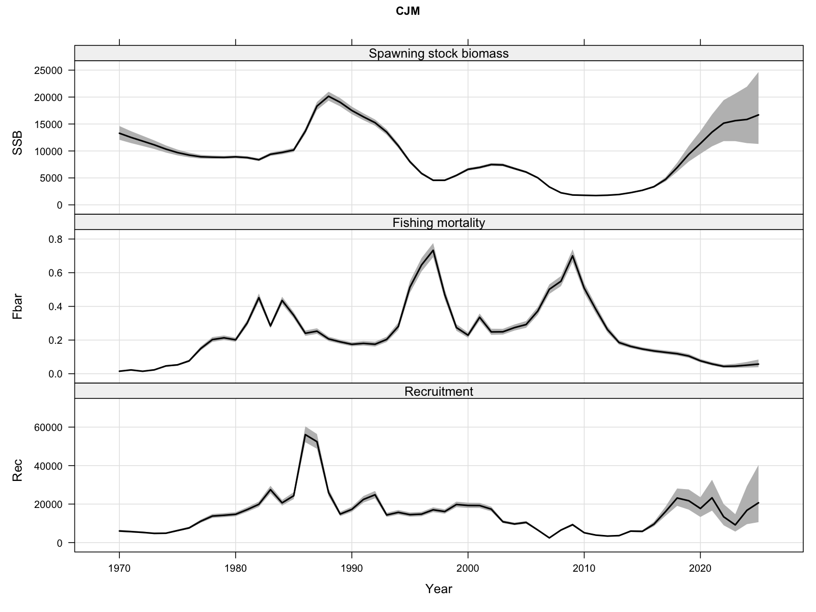
3.1 Stock trajectory
The full state-space trajectory with 95% confidence intervals. Recruitment, SSB, and mean F are estimated jointly with their process uncertainty.
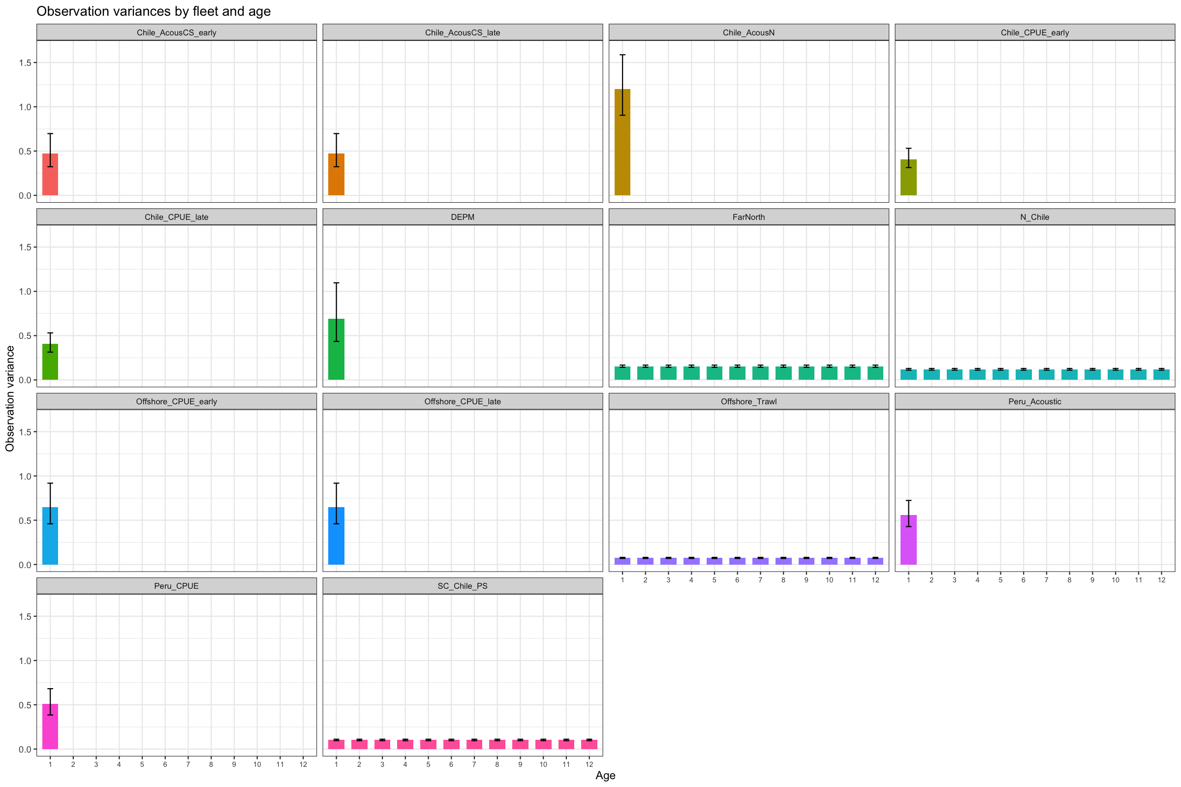
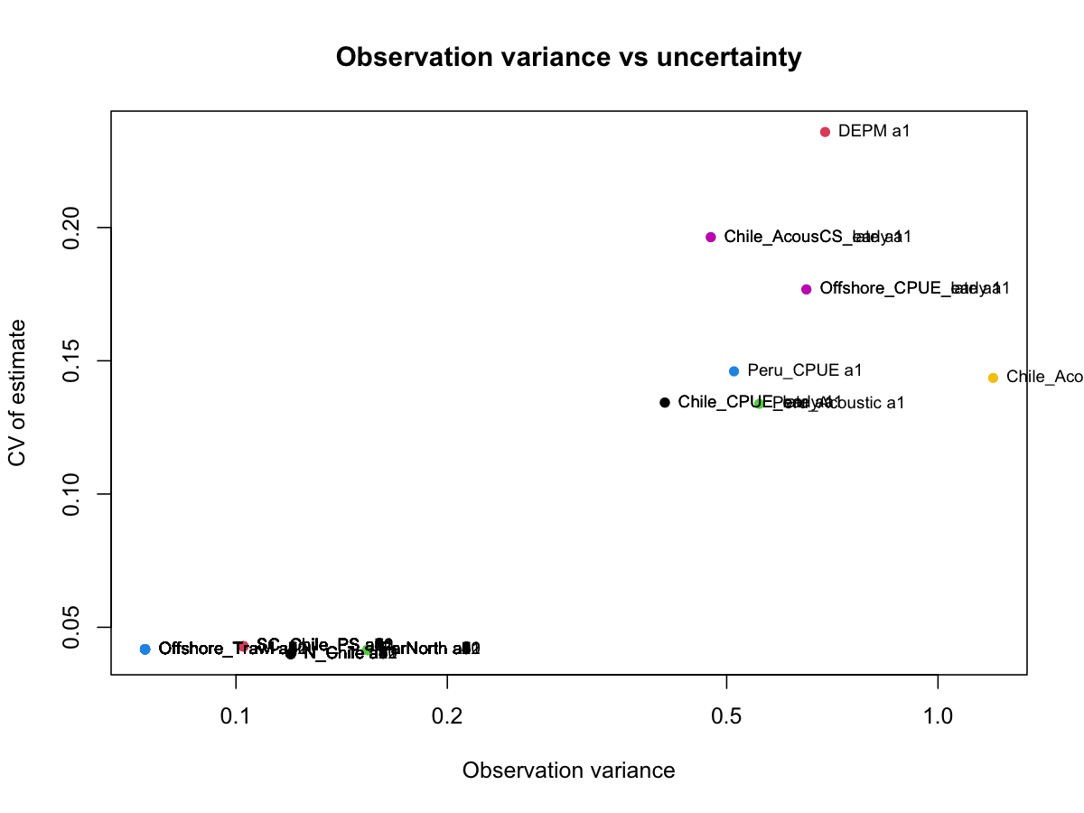
3.2 Observation variances
SAM estimates observation variances internally. Small values indicate a data source is given high weight; large values indicate the model discounts that source. All catch datasets are given high weight with the offshore trawl receiving highest weight. The ratio of observation variance to coefficient of variation (CV) reflects precision versus consistency. Generally, one doesn’t want to observe low observation variance with high CVs and vice versa, indicating inappropriate model fit.
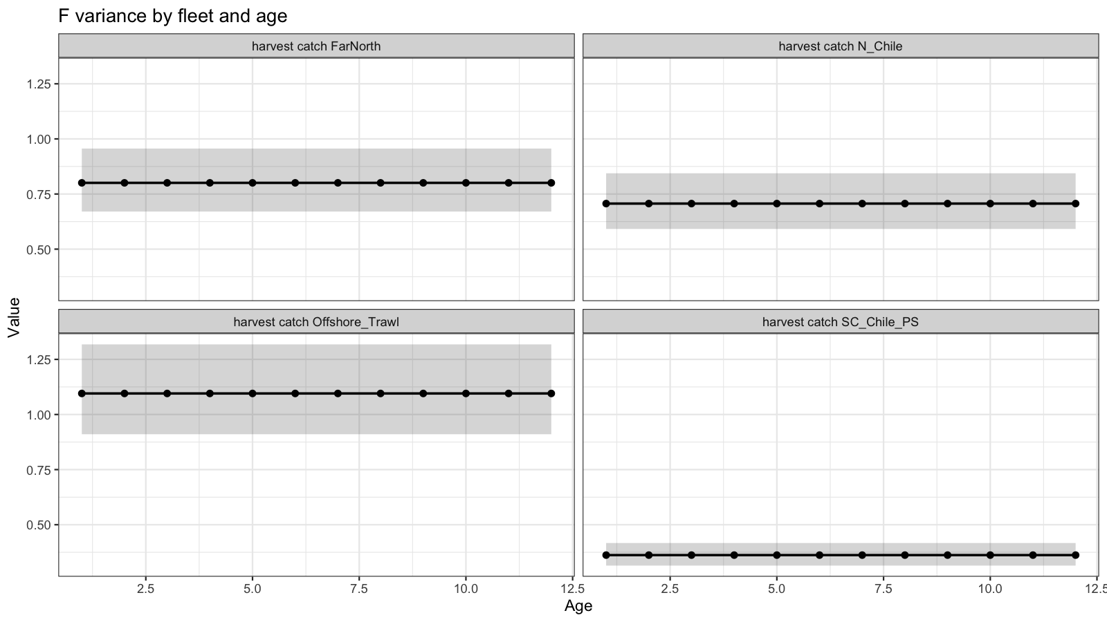
3.3 F variance parameters
Age-coupled F parameters control how smoothly selectivity varies across ages within each fleet. Panels show the estimated variance for each age group. In general, the best fitting model showed very similar variance across all ages. The South Central fleet showed lowest variability in F over time while the Offshore fleet showed highest variability.
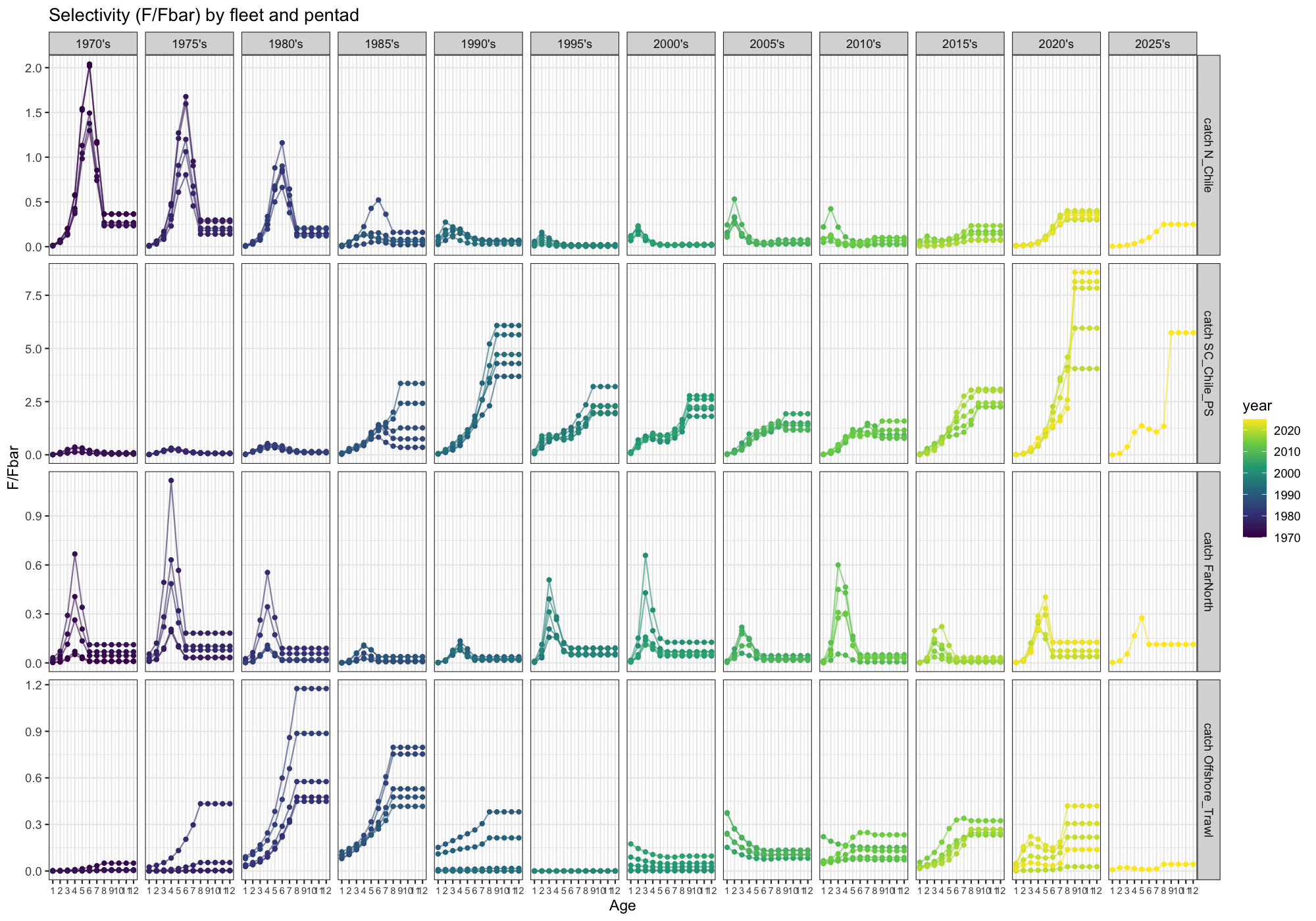
3.4 Selectivity
Selectivity is expressed as F/Fbar at each age and fleet, grouped by five-year periods to show temporal trends. Changes in shape over time may indicate non-stationarity in fleet behaviour or stock demography. There is substantial change in all fleets from relatively dome shaped to increasing and vice versa. The model estimates very high selection at oldest ages in the South Central fleet which is not expected to be driven by high mortality but probably due to a lack of availability.
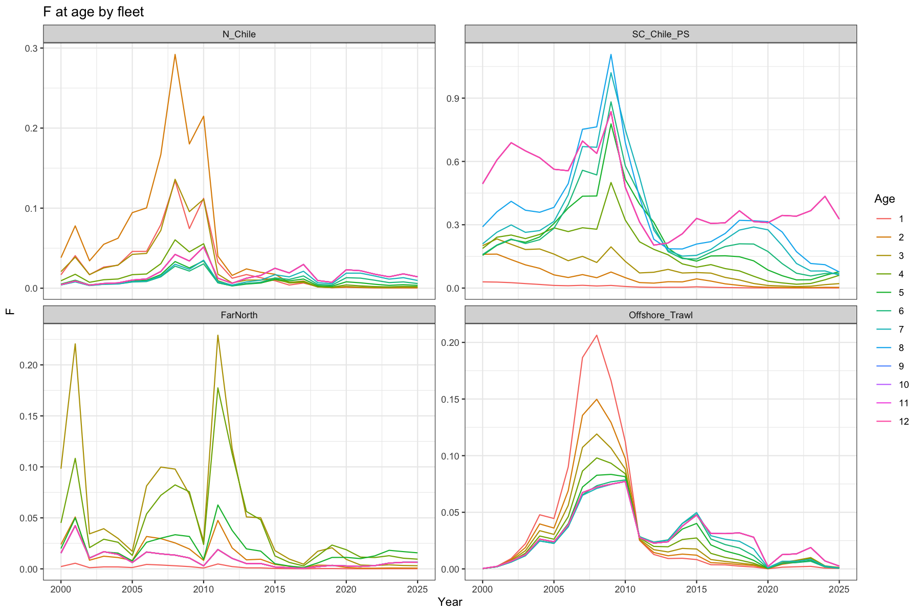
3.5 Fishing mortality at age
Fleet-specific F at age since 2000. Each panel corresponds to one of the four catch fleets.
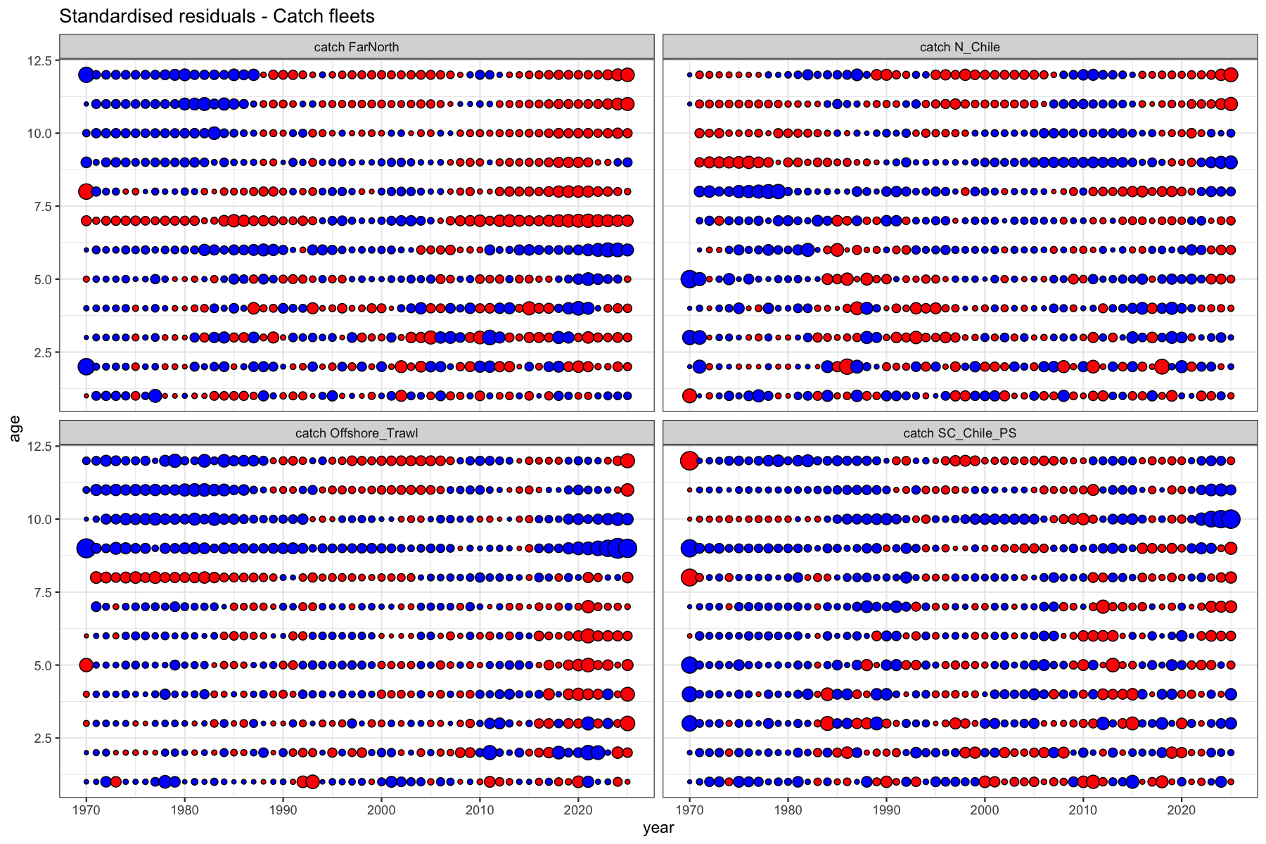
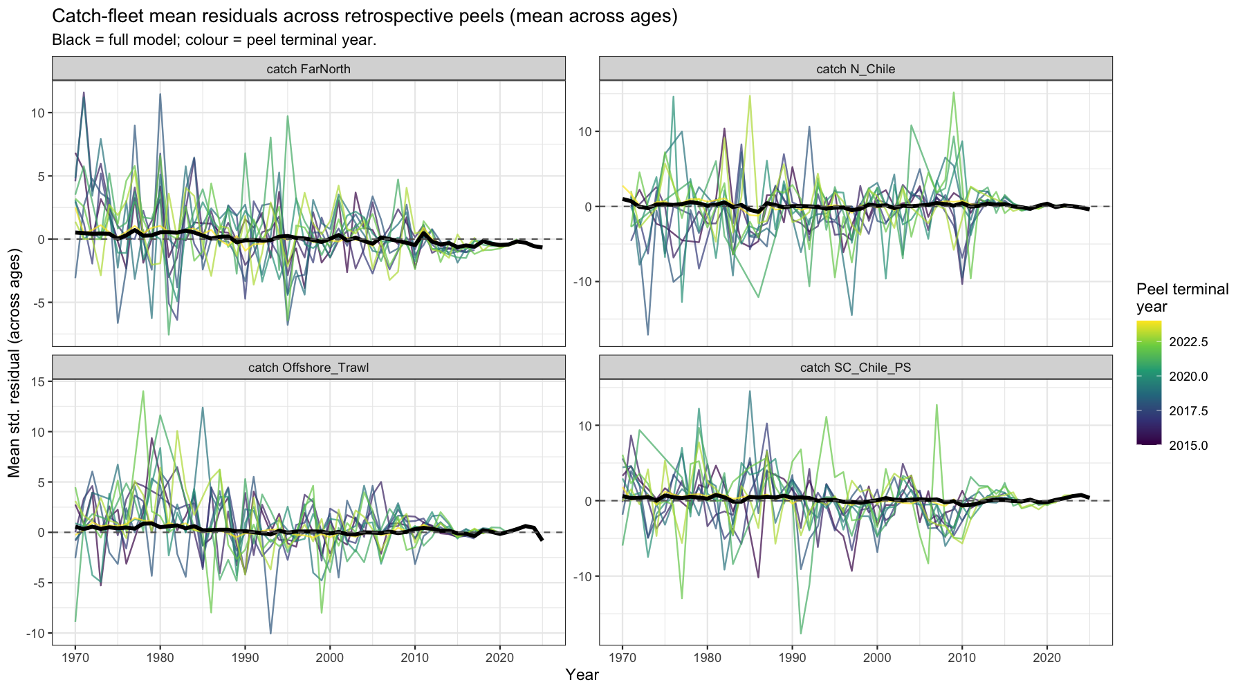
3.6 Catch residuals
Standardised residuals of the log-normal catch observation equation. Bubble area is proportional to the magnitude of the residual; blue = positive, red = negative. Systematic patterns (diagonal bands = cohort, horizontal bands = age, vertical bands = year effect) indicate model misspecification. There are substantial bands to be seen by age in the FarNorth fleet (age 6+), and the Offshore trawl (age 8+).
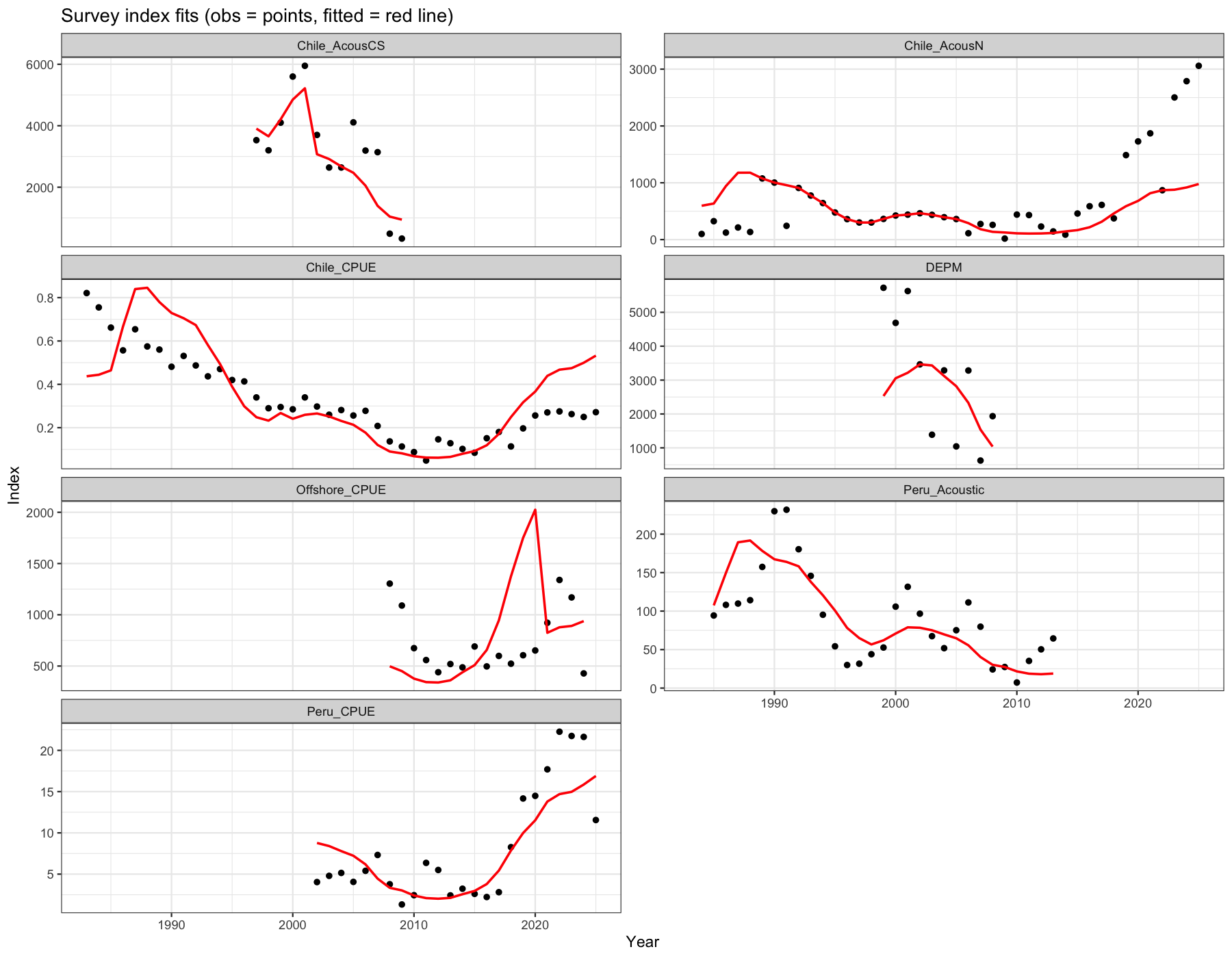
3.7 Survey index fits
Observed biomass index values (points) against model-predicted values (red line) for each survey. Persistent bias in a subset of years suggests time-varying catchability. There is considerably misfit for most of the indices. Especially pronounced are the misfits for Acoustic North, The Chilean CPUE, offshore CPUE and Peruvian CPUE.
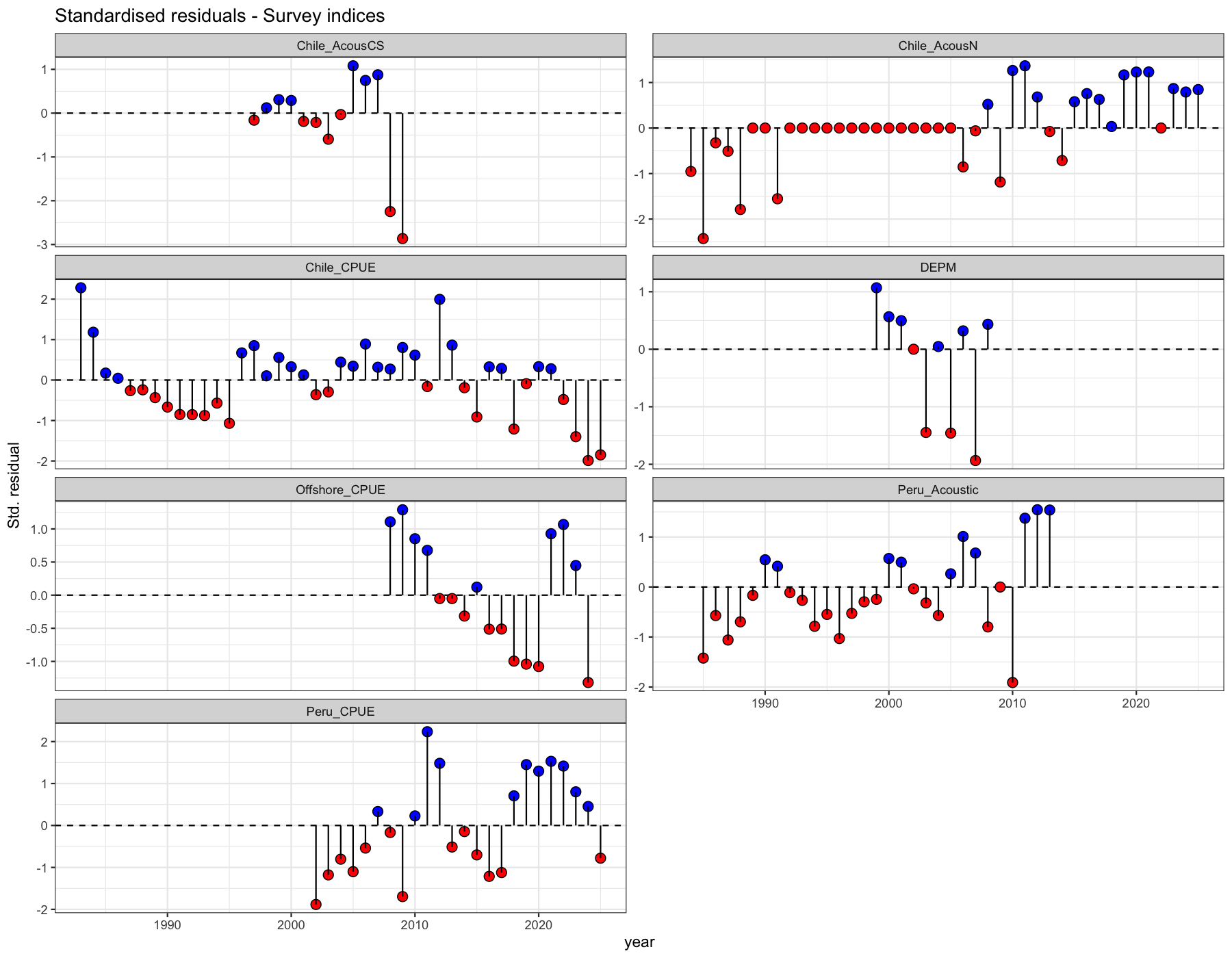
3.8 Survey residuals
Lollipop residual plot for survey biomass indices. A trend in residuals (e.g. positive early years and negative late years) indicates that SAM’s fixed-\(q\) assumption is violated for that survey.
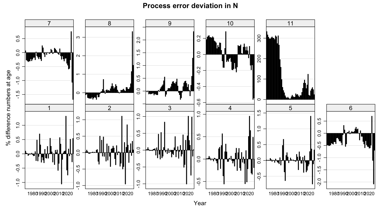
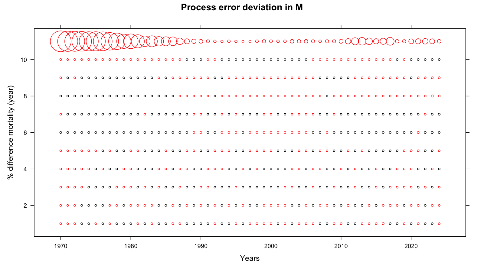
3.9 Process error
The process-error plots show the estimated deviation in log-numbers (top) and log-mortality (bottom) by age and year. Large process errors indicate years where the model needed to absorb information that the deterministic population projection could not explain. From age 6+ there are substantial temporal patterns with age 6 & 7 being opposite in sign from age 8 & 9 which may reflect issues with age reading. There is a general tendency to overestimate older ages.
3.10 Correlation matrix
The parameter correlation matrix provides a summary of structural collinearity in the model. There is high correlation between the between-age correlation (itrans_rho) in the F states and the variance parameters (logSdLogFsta) as s well as within the variance parameters. All other correlations are low.

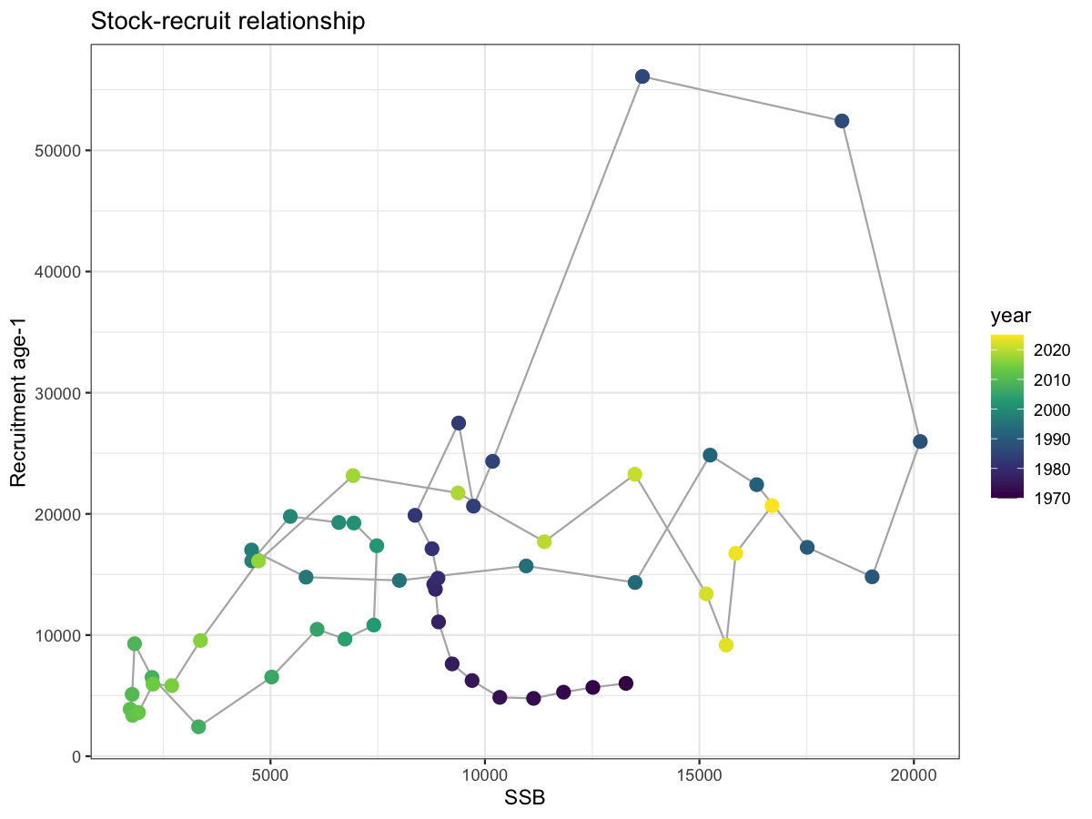
3.11 Stock-recruit relationship
The SSB–recruitment scatter provides a visual check on plausible stock dynamics. The absence of a strong Beverton-Holt or Ricker relationship is expected for short-lived pelagic species where recruitment is highly variable. Points coloured by year; path shows chronological sequence.
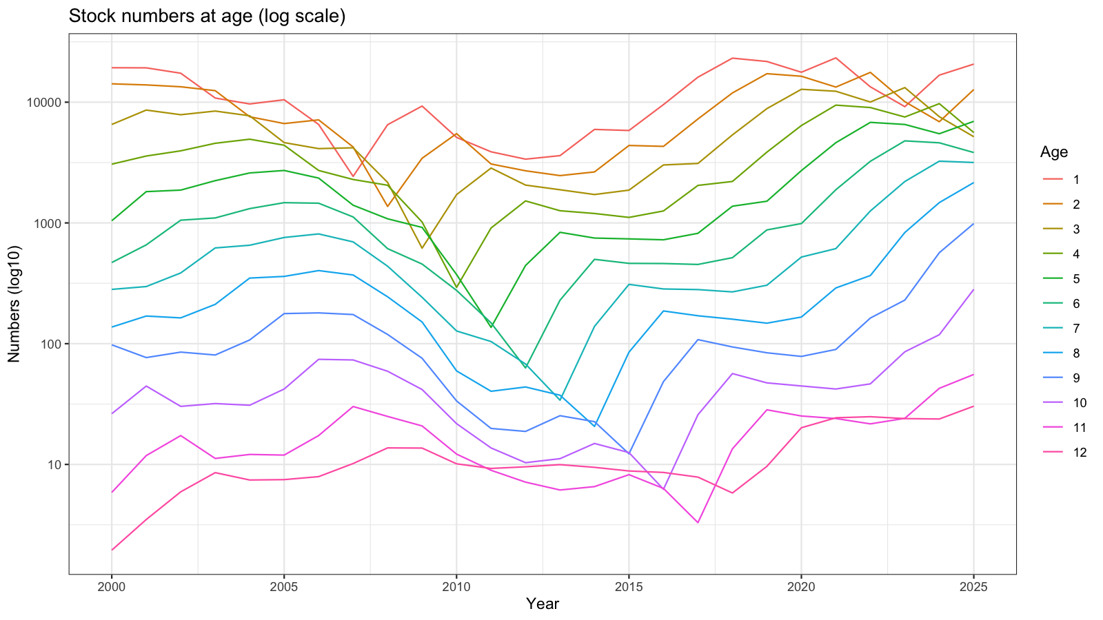
3.12 Numbers at age
Model-estimated stock numbers at age on a log scale since 2000. Parallel lines indicate stable age structure; divergence highlights cohort events or shifts in F.
4 Retrospective Analysis
Retrospective analyses sequentially remove the most recent year of data and re-fit the model. A systematic upward or downward revision of SSB or Fbar in the terminal year indicates a retrospective pattern, quantified by Mohn’s \(\rho\) (Mohn 1999). In general, retrospective patterns are reasonable for SSB (which is estimated with large uncertainty) and F.
\[ \rho = \frac{1}{n}\sum_{p=1}^{n}\frac{\hat{\theta}_{T-p,T-p} - \hat{\theta}_{T-p,T}}{\hat{\theta}_{T-p,T}} \]
where \(\hat{\theta}_{T-p,T-p}\) is the terminal-year estimate in the peel ending at year \(T-p\) and \(\hat{\theta}_{T-p,T}\) is the full-model estimate for the same year. Values of \(|\rho| > 0.20\) for SSB or \(|\rho| > 0.30\) for F are commonly considered problematic (Mohn 1999).
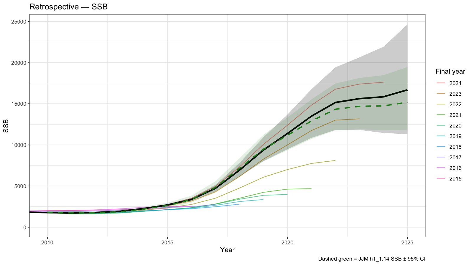
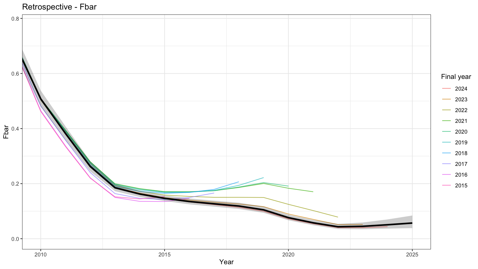
Mohn's rho
  SSB : -0.3889
  Fbar: 0.6556
4.1 In-depth retrospective diagnostics
Large retrospective patterns can arise from several sources: (i) re-estimation of catchability and observation-variance parameters as data are added; (ii) high-influence observations that cause the model to re-interpret earlier years once the terminal year is included; or (iii) surveys whose residual structure changes systematically as more data are appended. The following four diagnostics, run with residuals enabled in each retrospective peel, help identify which mechanism is dominant.
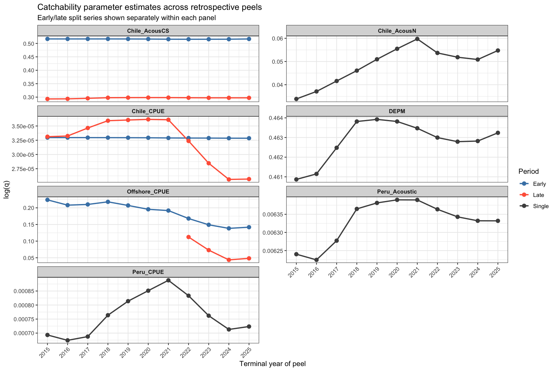
4.1.1 Catchability across peels
Catchability (\(\log q\)) is re-estimated in each peeled model. A stable \(\log q\) across peels indicates that the parameter is identified by the bulk of the time-series and is not being pulled by a small number of terminal-year observations. Large drifts — particularly in the most recent peels — suggest that new data are revising the model’s view of that survey’s relationship to biomass, which in turn propagates into a retrospective SSB revision. Especially the acoustic North and Peruvian CPUE show consistent trends in estimated catchability. In both cases, catcahbility increases meaning that the indices ‘see’ more fish. Declines are visible for the Offshore CPUE and the Chilean CPUE.
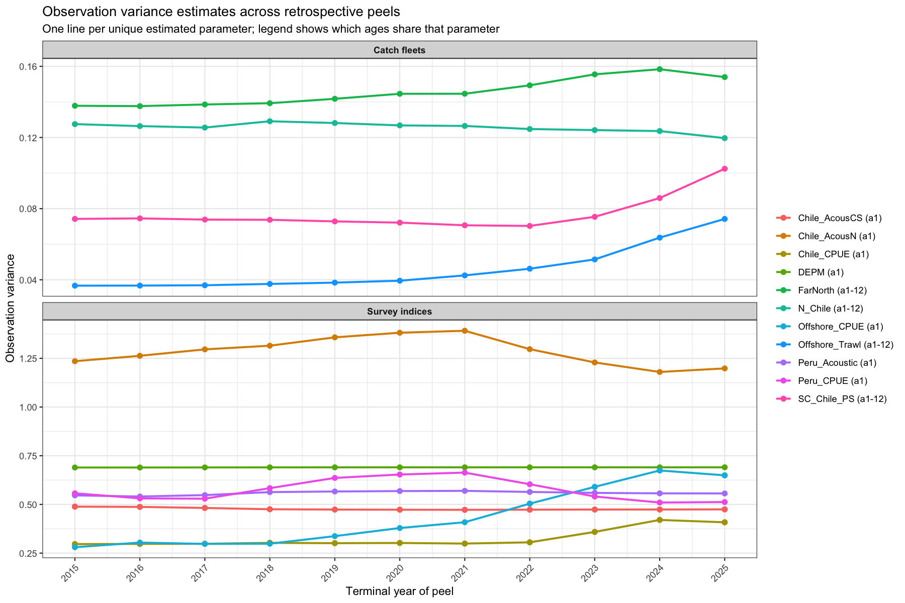
4.1.2 Observation variance across peels
Observation-variance (\(\sigma^2\)) parameters govern how much weight is placed on each data source. If \(\sigma^2\) for a survey drifts as years are removed, it signals that the noise structure inferred from recent data differs from the historical period — often a sign of a trend in data quality or catchability that the model absorbs into the variance estimate rather than the mean. The observation variance of the offshore and South Cental fishery has increased considerably over the past 5 years, but are still estimated at low levels. There seems to be some model instability which shows as sudden drops in observation variance for the Far North fleet.
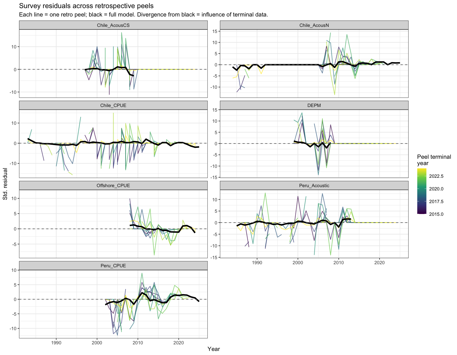
4.1.3 Survey residual spaghetti
Each line shows the standardised residuals of a survey for all years from one retrospective peel. The black line is the full model. If residuals in the middle of the time-series shift between peels, earlier data are being re-interpreted as terminal observations change — a structural conflict between that survey and others. If only the most terminal years shift, the pattern is consistent with normal retrospective behaviour driven by low information content at the data edge.
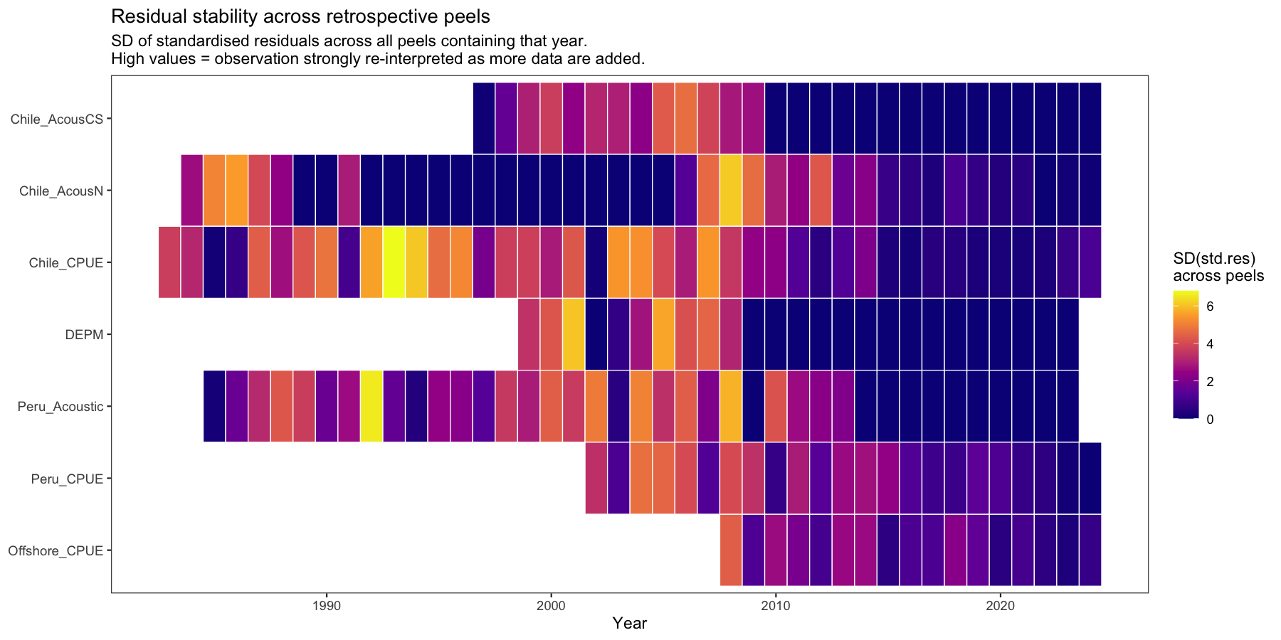
4.1.4 Residual stability heatmap
For each survey and year, the standard deviation of the standardised residual across all peels that included that year is computed. A year with high SD is re-interpreted substantially each time a new year of data is added — i.e. it has high leverage on the model trajectory. Years and surveys with consistently high SD are the primary suspects driving the retrospective pattern.
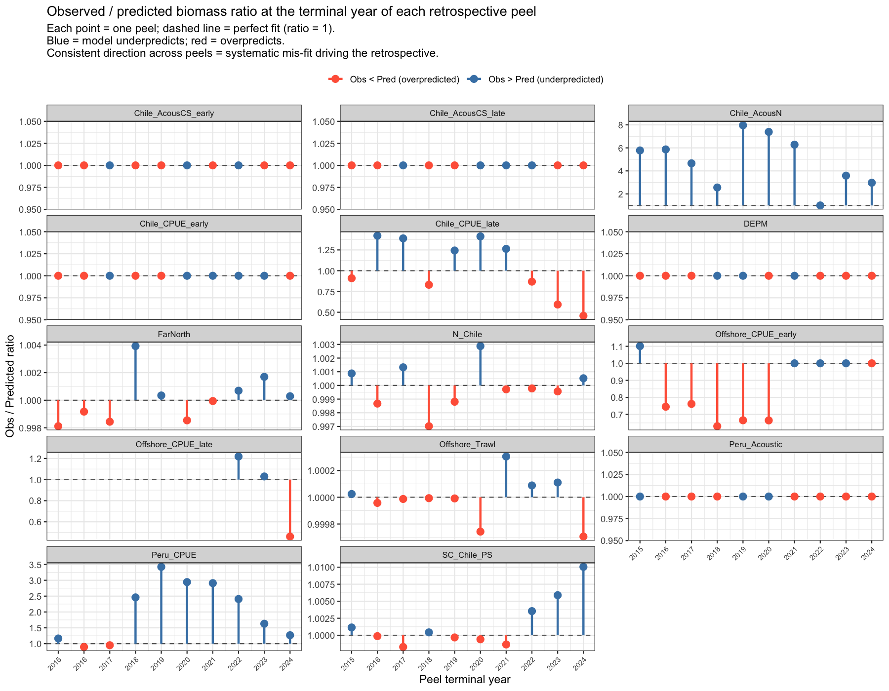
4.1.5 Terminal-year residuals: drivers of the retrospective pattern
The retrospective pattern arises because the model mis-fits certain observations at the terminal year of each peel. The plot below shows, for each fleet and each peel, the ratio of the observed to model-predicted biomass at that peel’s terminal year. A ratio consistently above 1 (blue) means the model persistently underpredicts that fleet’s terminal observation — causing it to revise the stock trajectory upward when a new year is added, which produces a negative Mohn’s ρ for SSB. The reverse applies for ratios below 1 (red). Surveys or catch fleets with consistently one-sided bars are the primary drivers of the retrospective.
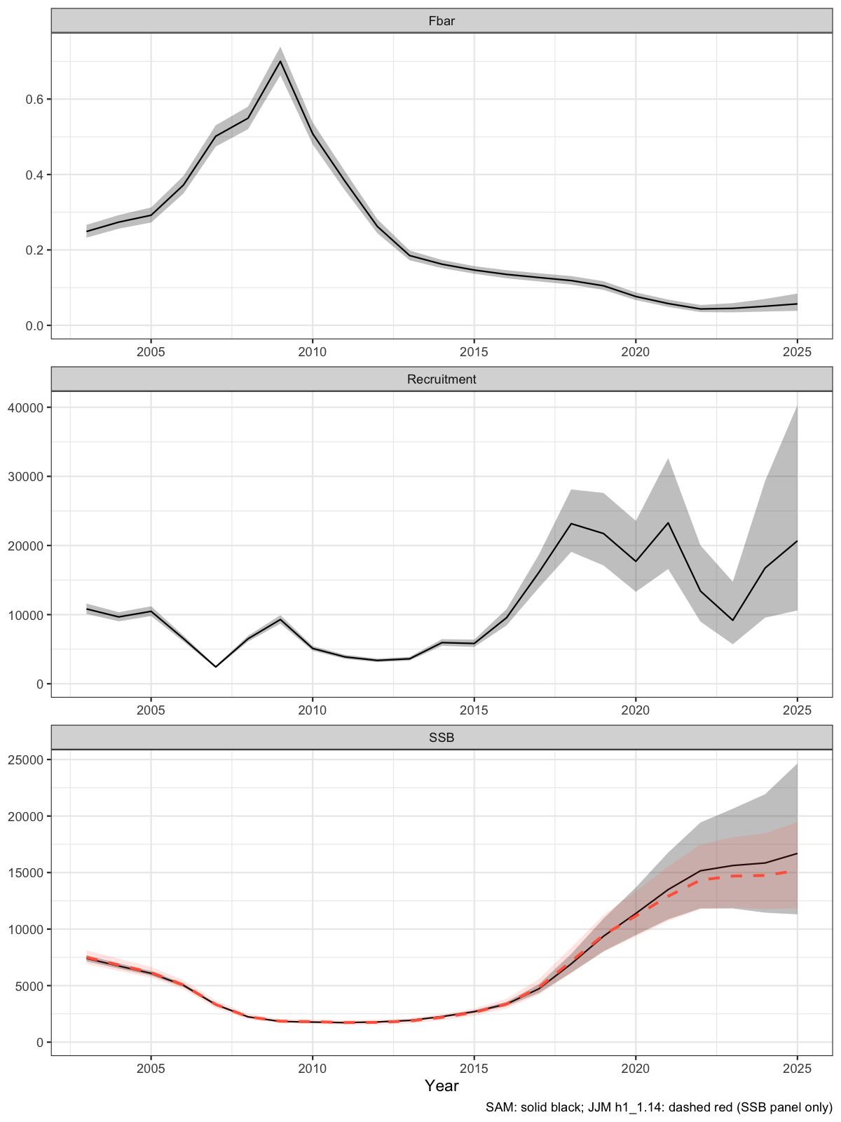
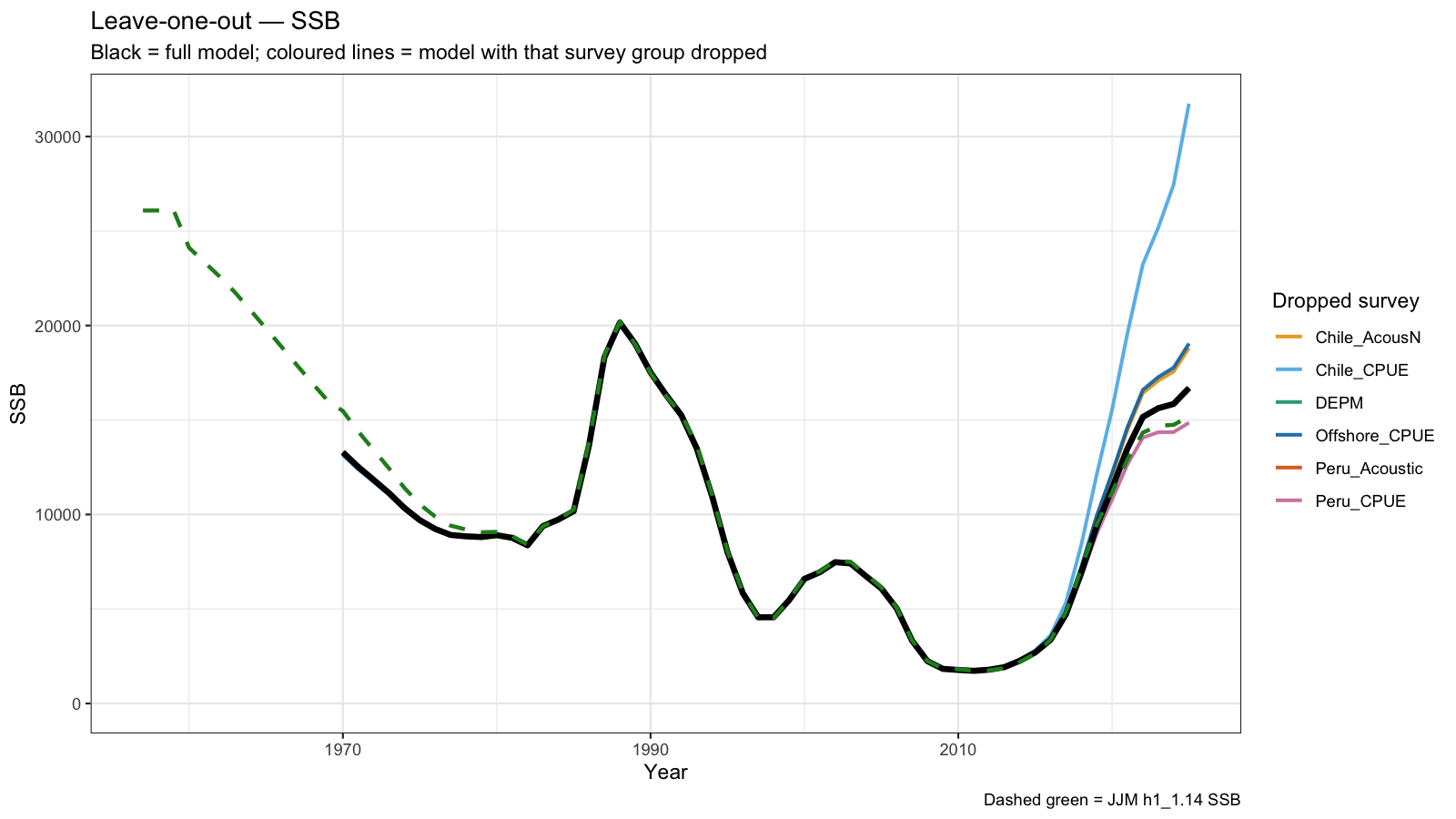
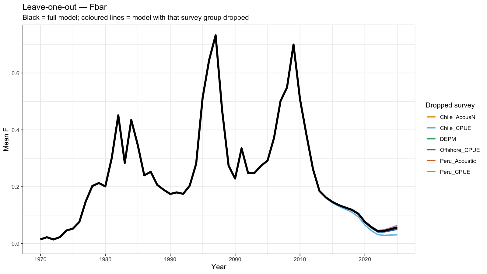
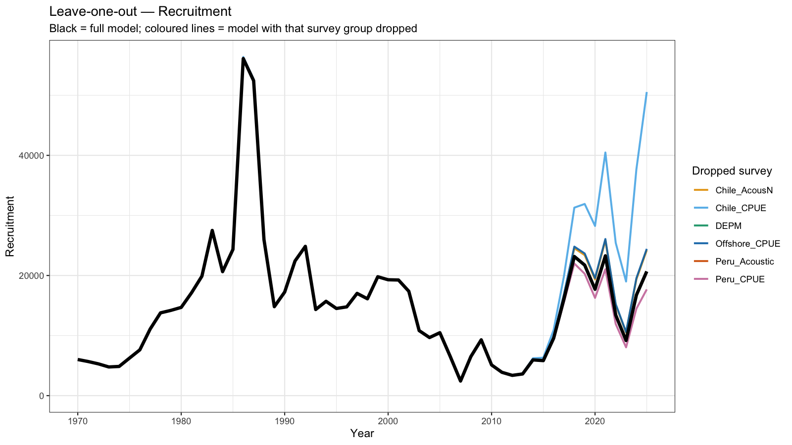
5 Leave-one-out Analysis
Leave-one-out (LOO) analysis refits the model seven times, each time omitting one survey group entirely. For the three surveys with JJM q-break years (Chile_AcousCS, Chile_CPUE, Offshore_CPUE), both the early and late sub-series are dropped together so that each LOO run represents a genuine removal of that data source.
The resulting SSB, Fbar, and recruitment trajectories are overlaid on the full model estimate. A large shift when a survey is dropped indicates that the model is strongly influenced by that data source — either because it carries substantial information or because it is in conflict with other inputs. Surveys whose removal causes little change are relatively redundant given the remaining data.
6 Catchability Diagnostics
Fixed catchability (\(q\)) is one of the most consequential assumptions in any assessment model. If the true \(q\) of a survey changes over time — due to changes in gear efficiency, stock distribution, or survey design — the model will accumulate systematic residuals. The following diagnostics are designed to detect and characterise such trends.
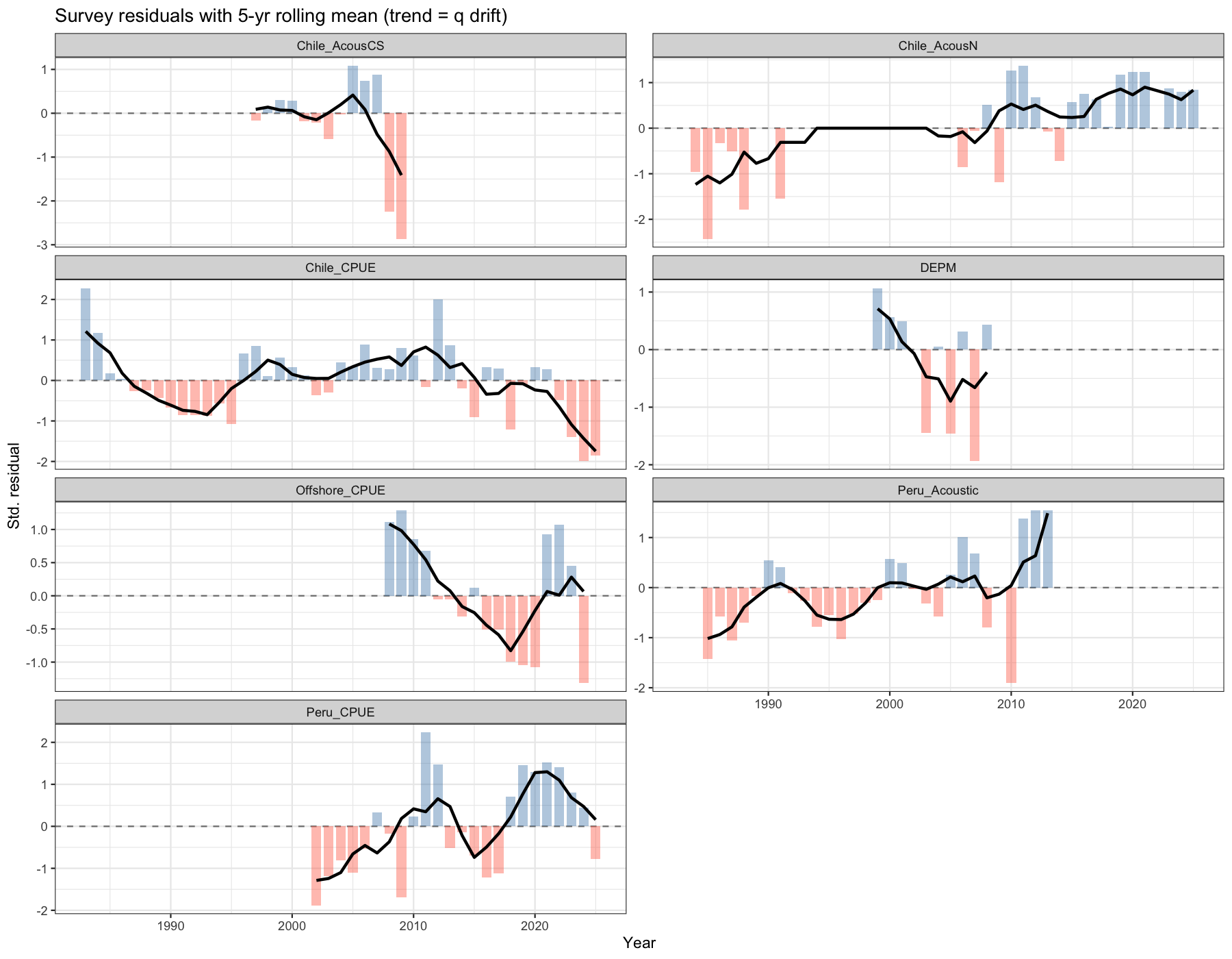
6.1 Rolling residuals and catchability drift
A five-year rolling mean of standardised residuals reveals slow shifts in effective catchability. Persistent positive residuals indicate the model is under-predicting the survey (i.e. \(q\) is in reality increasing), and vice versa. The figure clearly shows that several indices suffer from trends in residuals, specifically the the Chilean CPUE, offshore CPUE, Peruvian Acoustic.
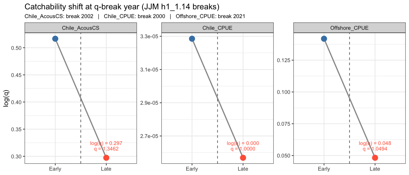
6.2 Catchability shift at break years
The JJM h1_1.14 control file assigns discrete q-break years to three indices (Chile_AcousCS: 2002, Chile_CPUE: 2000, Offshore_CPUE: 2021). To honour these structural breaks, each of these indices is split into an early and a late sub-series in SAM, with the two sub-series sharing the same observation variance parameter but receiving independent catchability estimates. The figure below shows the estimated log(q) for the early and late periods; a large shift indicates that the survey efficiency or stock availability changed substantially at the break year.
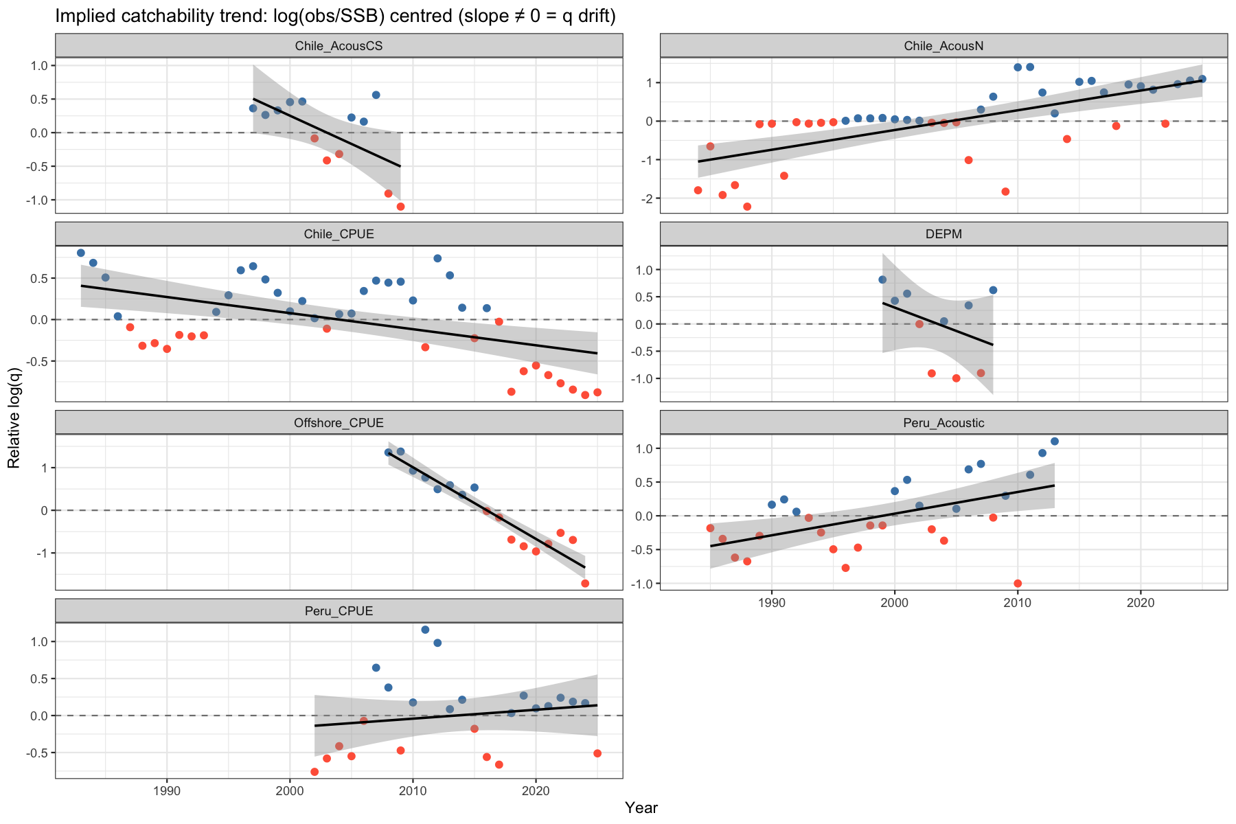
6.3 Implied catchability trend
The quantity \(\log(I_t) - \log(\hat{B}_t)\) is proportional to \(\log(q_t)\). Centring this series by its mean isolates the relative change in \(q\) over time. A significant linear trend (shown in grey) indicates that the constant-\(q\) assumption is violated. Only the Chilean Acoustic CS, the DEPM and the Peruvian CPUE show no significant trend.
6.4 Runs test
The Wald-Wolfowitz runs test (Methot and Wetzel 2013) evaluates whether the signs of residuals are distributed randomly. Significantly too few runs (p < 0.05) indicates a non-random pattern, most commonly caused by time-varying catchability or model misspecification.
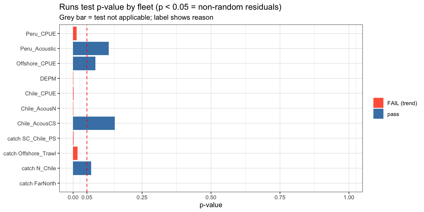
| fleet | n | n_runs | expected_runs | z | p_value | result |
|---|---|---|---|---|---|---|
| catch N_Chile | 56 | 20 | 26.1 | -1.841 | 0.0656 | pass |
| catch SC_Chile_PS | 56 | 15 | 25.4 | -3.233 | 0.0012 | FAIL (trend) |
| catch FarNorth | 56 | 12 | 29.0 | -4.585 | 0.0000 | FAIL (trend) |
| catch Offshore_Trawl | 56 | 16 | 23.0 | -2.407 | 0.0161 | FAIL (trend) |
| Chile_AcousCS | 13 | 5 | 7.5 | -1.435 | 0.1512 | pass |
| Chile_AcousN | 42 | 12 | 8.3 | 3.445 | 0.0006 | FAIL (trend) |
| Chile_CPUE | 43 | 12 | 22.4 | -3.225 | 0.0013 | FAIL (trend) |
| DEPM | 10 | 8 | 4.6 | 3.334 | 0.0009 | FAIL (trend) |
| Peru_Acoustic | 29 | 10 | 13.4 | -1.518 | 0.1291 | pass |
| Peru_CPUE | 24 | 7 | 12.9 | -2.488 | 0.0129 | FAIL (trend) |
| Offshore_CPUE | 17 | 6 | 9.5 | -1.745 | 0.0810 | pass |
7 Fleet Conflict and Compensation Diagnostics
When multiple fleets and surveys contribute information to the same population trajectory, they may provide conflicting signals. SAM’s internal weighting resolves conflicts by down-weighting inconsistent sources, but residual patterns can still reveal the nature of the tension.
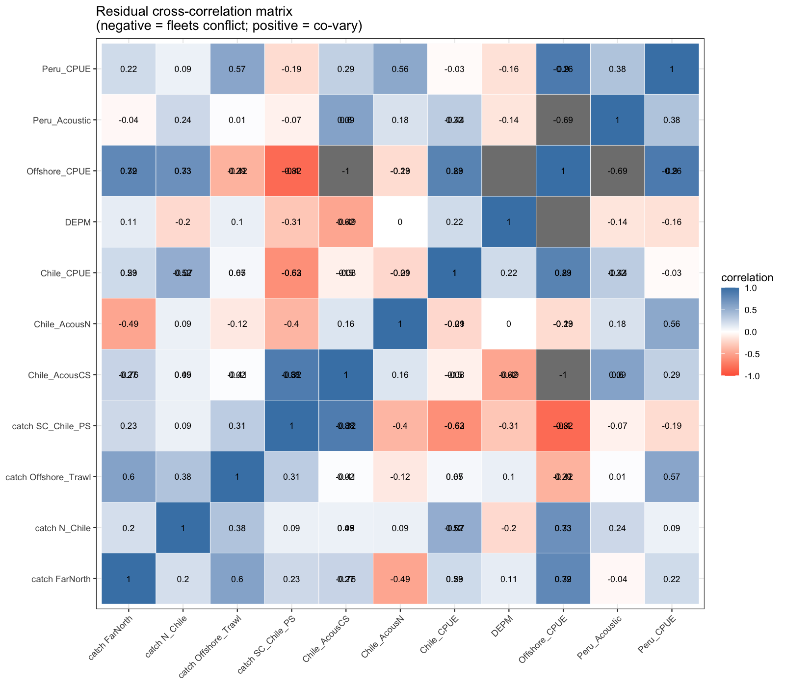
7.1 Residual cross-correlation matrix
The cross-correlation of annual (mean) residuals between all fleets identifies structural conflicts. A strong negative correlation between two fleets means one over-predicts systematically when the other under-predicts — a diagnostic signal for fleet compensation. Positive correlations suggest fleets respond coherently to the same environmental or stock signal. Especially the offshore CPUE contradicts in trend with the Chilean SC catch data, although the correlation with the Chilean SC CPUE is high.
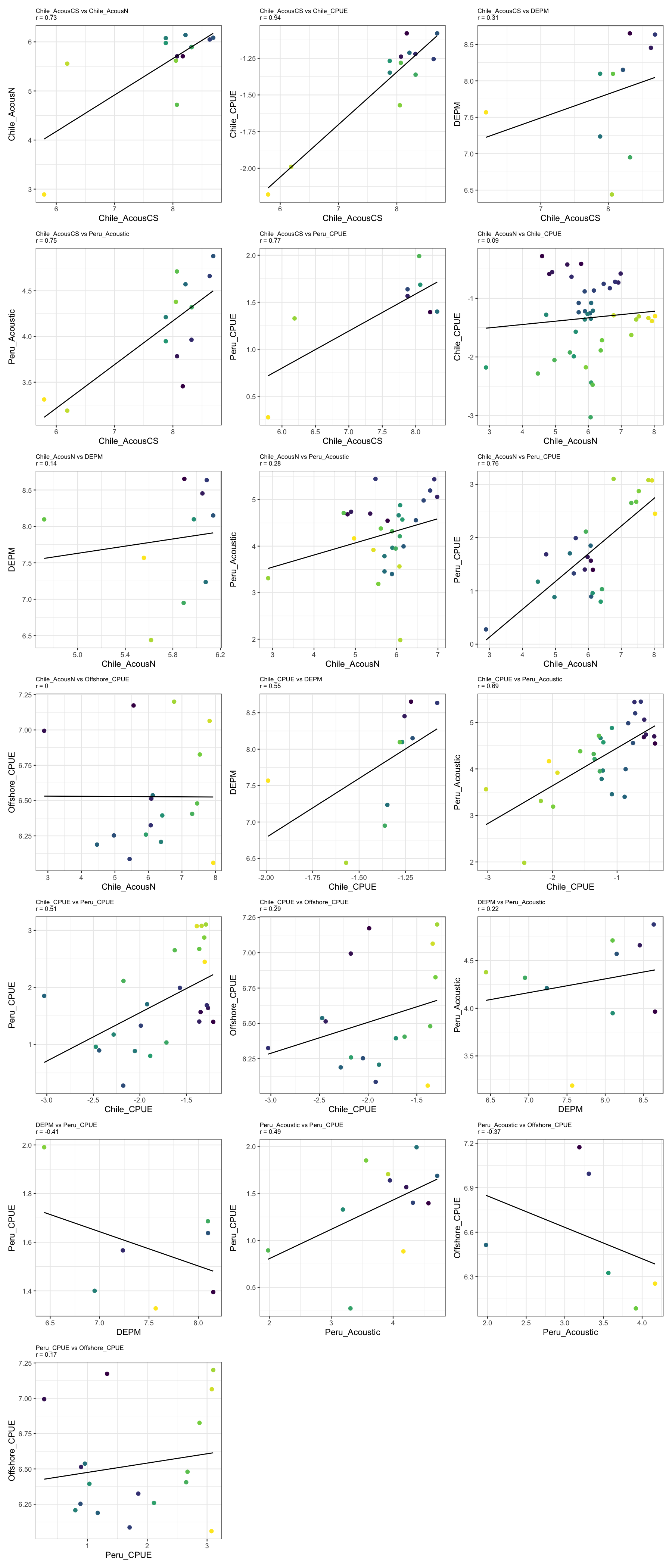
7.2 Pairwise survey index scatter
Plotting pairs of survey indices over shared years shows whether surveys agree on the direction and magnitude of stock change. Diverging trends or low correlations indicate that surveys sample different components of the stock or are affected by different sources of variability.
7.3 Cohort tracking across catch fleets
The same cohort should be detectable across all catch fleets as it ages through the population. If catch-at-age data from different fleets show diverging relative abundance for the same cohort at the same age, it indicates either gear selectivity conflicts, spatial overlap differences, or data inconsistencies. There is very poor cohort tracking capabilities for the different catch@age data. For example, the 2018 cohort is picked up markedly different by 3 out of the 4 fleets.
8 Productivity Analysis
8.1 Rationale
The Beverton-Holt stock-recruitment relationship describes how spawning biomass (SSB) translates into future recruitment. The steepness parameter \(h\) is the fraction of unfished recruitment \(R_0\) that is produced at 20% of unfished SSB (\(B_0\)):
\[ R = \frac{0.8\,R_0\,h\,\text{SSB}}{0.2\,B_0(1-h) + (5h-1)\,\text{SSB}} \quad\equiv\quad R = \frac{a\,\text{SSB}}{b + \text{SSB}}, \quad h = \frac{0.2(b + B_0)}{b + 0.2\,B_0} \]
where \(B_0\) is approximated by the maximum observed SSB. High steepness (\(h > 0.8\)) indicates low compensation — recruitment is nearly independent of spawning biomass.
A change in steepness over time signals a shift in stock productivity that is not captured by the primary assessment model (JJM uses fixed life-history parameters). Such shifts can arise from regime changes, density-dependent effects at low stock size, or environmental shifts affecting larval survival.
8.2 Method
Beverton-Holt curves are fitted by weighted nonlinear least squares, using uncertainty in the SAM recruitment estimate as observation weights:
\[ w_t = \frac{1}{\hat{\sigma}^2_{\log R_t}}, \qquad \hat{\sigma}_{\log R_t} \approx \frac{\text{CI}_{97.5} - \text{CI}_{2.5}}{4\,R_t} \]
Change points are found by exhaustive search over all candidate break years (minimum 10 years per segment). The improvement in total weighted residual SS when adding a break is tested with an \(F\)-test (2 additional parameters per break). A second break is only searched if the first is significant at \(p < 0.05\).
Beverton-Holt productivity analysis
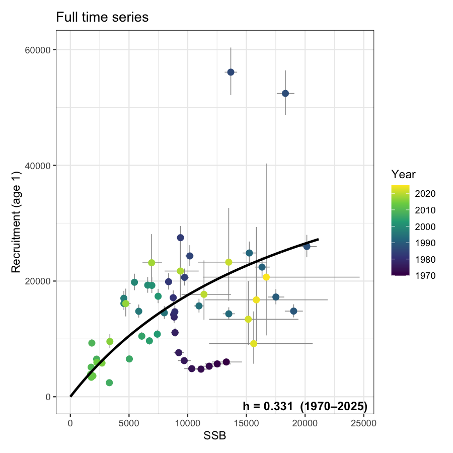
B0 reference (max observed SSB): 20149
Full series: h = 0.331 (1970-2025)
1-break test: break year 1993, p = 0.3647 [not significant]
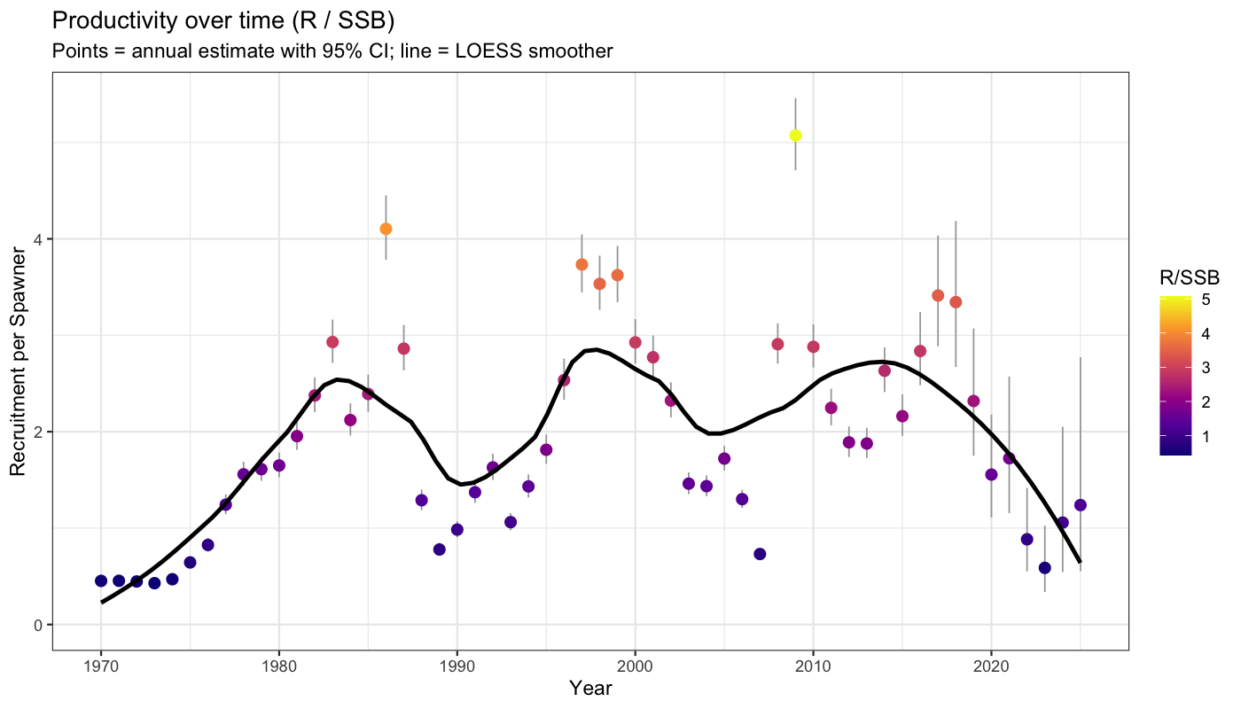
8.3 Productivity over time
Annual productivity (R/SSB) with 95% confidence intervals propagated from SAM uncertainty in both recruitment and SSB via the delta method on the log scale: \(\text{SE}_{\log(R/\text{SSB})} \approx \sqrt{\text{SE}^2_{\log R} + \text{SE}^2_{\log \text{SSB}}}\). A LOESS smoother highlights the long-term trend without imposing a parametric form.
8.4 Stock-recruit panels
Up to three panels are shown depending on how many break points are statistically supported. The legend of each multi-period panel includes the estimated steepness for that period. Error bars show 95% confidence intervals from SAM on both SSB (horizontal) and recruitment (vertical).
9 Selectivity Block Suggestions for JJM
9.1 Rationale
JJM requires the user to pre-specify constant-selectivity blocks: periods within which selectivity-at-age is assumed to be time-invariant. In practice these blocks are set based on expert knowledge of fleet changes, but there is no objective statistical criterion for where boundaries should fall.
SAM estimates selectivity annually through the random-walk F process. The trajectory of the annual selectivity shape (F/Fbar at age, normalised so the peak = 1) therefore provides an empirical signal of when selectivity changed significantly. A structural break in this trajectory is a principled suggestion for a new JJM block boundary.
9.2 Method
For each catch fleet:
- The normalised selectivity-at-age vector is extracted for every year from the SAM fit (shape only: F/Fbar at age, scaled so the peak age = 1).
- The dominant mode of temporal variation is captured by the first principal component (PC1) of the annual selectivity matrix.
- The PC1 time series is split into blocks using binary segmentation, with each year weighted by its relative catch (\(w_t = C_t / \max C\)). This ensures that periods with little fishing activity have minimal influence on where block boundaries are placed. Splits require \(p < 0.05\) (F-test) and at least five years per segment.
- Each detected breakpoint is assigned an importance score:
\[ \text{importance} = F_{\text{split}} \times \frac{\sum_{t \in \text{segment}} C_t}{C_{\text{total}}} \]
Breakpoints are ranked 1 (most important) downward: rank 1 should be kept even if the number of blocks is reduced; rank \(k\) can be dropped first. This allows a user to move from the full block structure to a simpler one by dropping the highest-numbered ranks. 5. Within-block variance, peak-selectivity age, and the percentage of total fleet catch in each block are reported as supporting statistics.
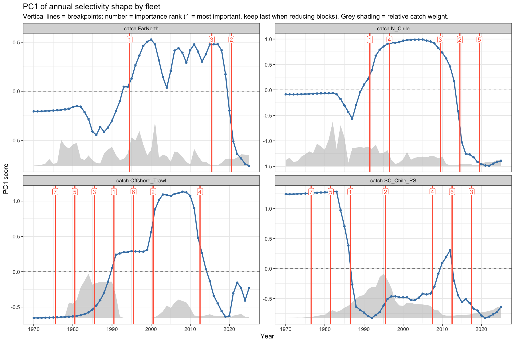
9.3 PC1 trajectories and block boundaries
The PC1 score over time reveals the dominant mode of selectivity change. Vertical red lines mark suggested block boundaries; the number is the importance rank (1 = most important). Grey shading behind the line shows the relative catch weight. To reduce the number of blocks, drop boundaries starting from the highest rank number.
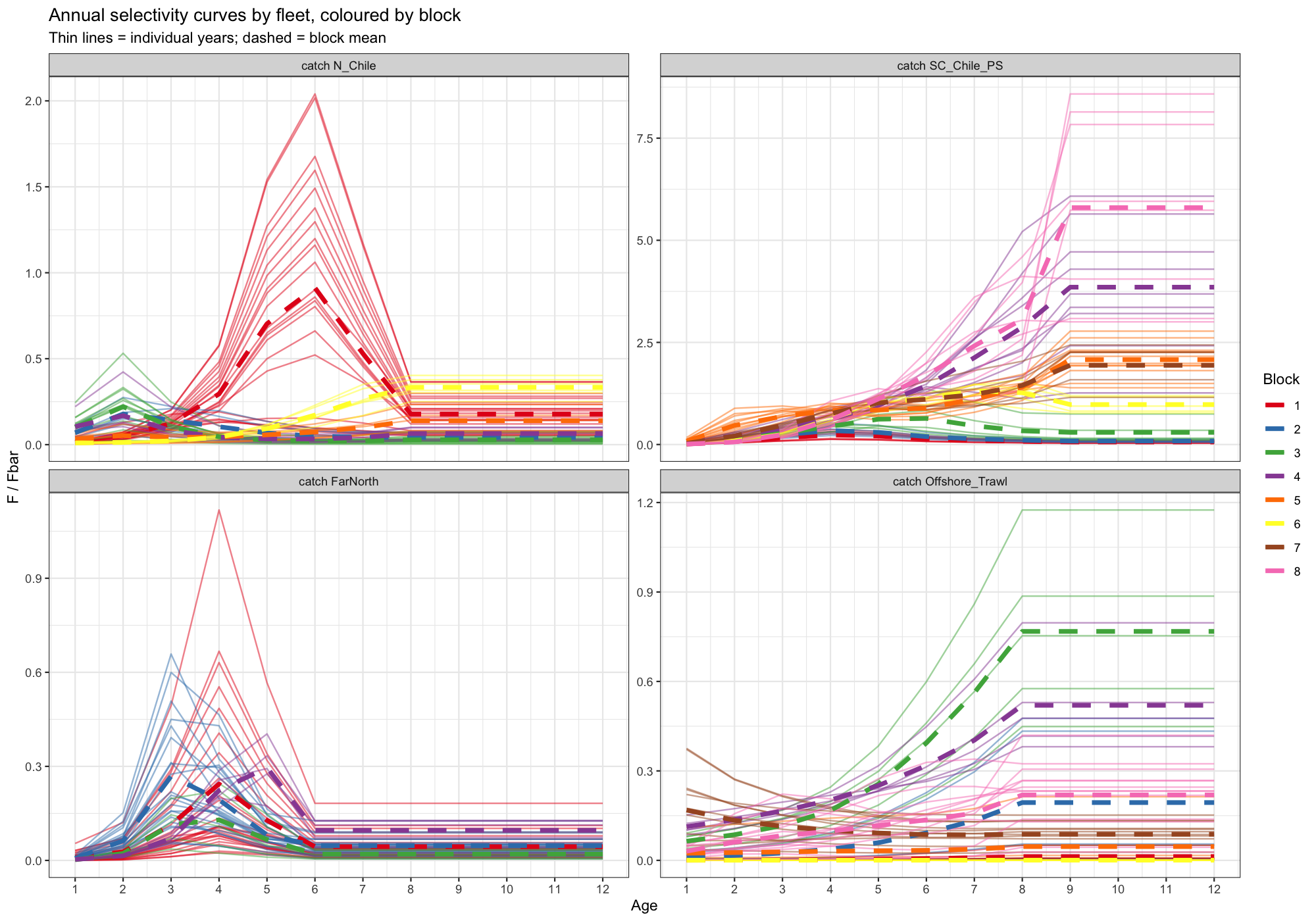
9.4 Selectivity curves by block
Individual annual selectivity curves are shown in the colour of their assigned block; the dashed line is the block mean. Blocks with tightly clustered curves support the constant-selectivity assumption; blocks where thin lines diverge strongly from the mean suggest that within-block variation may still be substantial.
9.5 Suggested block table
| Fleet | Block | Start | End | N years | Catch % | Peak age | Within-var. | Boundary rank | Rationale |
|---|---|---|---|---|---|---|---|---|---|
| catch N_Chile | 1 | 1970 | 1991 | 22 | 63.0 | 6 | 0.02544 | 1 | Initial block |
| catch N_Chile | 2 | 1992 | 1996 | 5 | 13.1 | 2 | 0.01529 | 4 | Peak age shifted 6 → 2 (13.1% of catch) |
| catch N_Chile | 3 | 1997 | 2009 | 13 | 16.4 | 2 | 0.00099 | 3 | Selectivity shape change (16.4% of fleet catch in block) |
| catch N_Chile | 4 | 2010 | 2014 | 5 | 2.3 | 2 | 0.02440 | 2 | Selectivity shape change (2.3% of fleet catch in block) |
| catch N_Chile | 5 | 2015 | 2019 | 5 | 1.1 | 8 | 0.00876 | 5 | Peak age shifted 2 → 8 (1.1% of catch) |
| catch N_Chile | 6 | 2020 | 2025 | 6 | 4.1 | 8 | 0.00113 | — | Selectivity shape change (4.1% of fleet catch in block) |
| catch SC_Chile_PS | 1 | 1970 | 1976 | 7 | 0.4 | 4 | 0.00001 | 7 | Initial block |
| catch SC_Chile_PS | 2 | 1977 | 1981 | 5 | 2.5 | 4 | 0.00001 | 5 | Selectivity shape change (2.5% of fleet catch in block) |
| catch SC_Chile_PS | 3 | 1982 | 1986 | 5 | 7.0 | 5 | 0.02234 | 1 | Selectivity shape change (7.0% of fleet catch in block) |
| catch SC_Chile_PS | 4 | 1987 | 1995 | 9 | 41.2 | 9 | 0.00980 | 2 | Peak age shifted 5 → 9 (41.2% of catch) |
| catch SC_Chile_PS | 5 | 1996 | 2007 | 12 | 33.3 | 9 | 0.00843 | 4 | Selectivity shape change (33.3% of fleet catch in block) |
| catch SC_Chile_PS | 6 | 2008 | 2012 | 5 | 3.7 | 7 | 0.00801 | 6 | Peak age shifted 9 → 7 (3.7% of catch) |
| catch SC_Chile_PS | 7 | 2013 | 2017 | 5 | 2.3 | 9 | 0.01082 | 3 | Peak age shifted 7 → 9 (2.3% of catch) |
| catch SC_Chile_PS | 8 | 2018 | 2025 | 8 | 9.4 | 9 | 0.02234 | — | Selectivity shape change (9.4% of fleet catch in block) |
| catch FarNorth | 1 | 1970 | 1994 | 25 | 40.3 | 4 | 0.00410 | 1 | Initial block |
| catch FarNorth | 2 | 1995 | 2015 | 21 | 48.6 | 3 | 0.01134 | 3 | Selectivity shape change (48.6% of fleet catch in block) |
| catch FarNorth | 3 | 2016 | 2020 | 5 | 3.1 | 3 | 0.00901 | 2 | Selectivity shape change (3.1% of fleet catch in block) |
| catch FarNorth | 4 | 2021 | 2025 | 5 | 8.0 | 5 | 0.00732 | — | Peak age shifted 3 → 5 (8.0% of catch) |
| catch Offshore_Trawl | 1 | 1970 | 1975 | 6 | 0.1 | 8 | 0.00000 | 7 | Initial block |
| catch Offshore_Trawl | 2 | 1976 | 1980 | 5 | 5.9 | 8 | 0.00001 | 5 | Selectivity shape change (5.9% of fleet catch in block) |
| catch Offshore_Trawl | 3 | 1981 | 1985 | 5 | 30.3 | 8 | 0.00022 | 3 | Selectivity shape change (30.3% of fleet catch in block) |
| catch Offshore_Trawl | 4 | 1986 | 1990 | 5 | 33.2 | 8 | 0.00534 | 1 | Selectivity shape change (33.2% of fleet catch in block) |
| catch Offshore_Trawl | 5 | 1991 | 1995 | 5 | 4.5 | 8 | 0.00009 | 6 | Selectivity shape change (4.5% of fleet catch in block) |
| catch Offshore_Trawl | 6 | 1996 | 2000 | 5 | 0.0 | 8 | 0.00163 | 2 | Selectivity shape change (0.0% of fleet catch in block) |
| catch Offshore_Trawl | 7 | 2001 | 2012 | 12 | 20.9 | 1 | 0.04161 | 4 | Peak age shifted 8 → 1 (20.9% of catch) |
| catch Offshore_Trawl | 8 | 2013 | 2025 | 13 | 5.1 | 8 | 0.02438 | — | Peak age shifted 1 → 8 (5.1% of catch) |
9.6 Caveats
- The analysis operates on SAM’s estimated selectivity, which itself carries uncertainty. Short blocks (< 5 years) or blocks separated by a weak PC1 shift should be treated with caution.
- SAM’s random-walk F tends to smooth selectivity; abrupt one-year anomalies visible in the raw data may be absorbed into the process error rather than reflected in the selectivity trajectory.
- The suggestions are a starting point. Fleet-specific information (gear changes, area closures, quota redistribution) should take precedence when it conflicts with the statistical signal.
10 Discussion
10.1 Utility of SAM as a diagnostic tool
The primary value of applying SAM alongside JJM is not to replace the primary assessment but to leverage SAM’s internal observation-variance estimation to identify data-weighting inconsistencies. Where SAM assigns a high observation variance to a particular fleet, it suggests that the fleet’s contribution to the likelihood is relatively small — a finding that may inform external weighting decisions in JJM.
The process-error plots (Section Section 3) are particularly informative: large process errors in specific age classes or years indicate that the deterministic population projection is insufficient to track the observed data, which may signal recruitment events, migration, or measurement issues not captured in the model structure.
10.2 Interpreting catchability diagnostics
The implied-\(q\) diagnostics (Section Section 6) should be interpreted with care for biomass-only surveys covering large and spatially heterogeneous stock distributions. The ratio \(\log(I_t) - \log(\hat{B}_t)\) conflates true catchability change with changes in stock distribution, survey coverage, and gear efficiency. A statistically significant trend in this quantity is a necessary but not sufficient condition for concluding that survey \(q\) has changed.
For the runs test, non-random residuals (p < 0.05) are common in long biomass survey series covering stocks with high interannual variability, particularly when the fixed-\(q\) model cannot fully describe index dynamics. These results should be treated as prompts for investigation rather than definitive evidence of model failure.
10.3 Fleet conflict and compensation
Negative entries in the residual cross-correlation matrix (Section 7.1) indicate that two fleets pull the model in opposite directions. If stock distribution shifts northward in some years, one survey will over-index while another under-indexes, even if total abundance is unchanged.
SAM resolves these conflicts through differential down-weighting, but the resolution implies that the “losing” fleet contributes less to the final trajectory estimate. Pairwise scatter plots (Section 7.2) and cohort tracking (Section 7.3) help identify which surveys are internally consistent with each other and which represent independent or contradictory signals.
10.4 Limitations of the SAM diagnostic
Several aspects of the JJM assessment cannot be directly evaluated through SAM:
- Length composition data are not used in the SAM fit. JJM uses both age and length compositions, and the interaction between the two likelihood components is an important source of information on the growth transition matrix.
- Biomass-index simplification: JJM surveys may be age-disaggregated or vulnerability-weighted, whereas the SAM diagnostic treats all indices as integrated biomass. This may absorb selectivity changes into the \(q\) term.
- Stock-recruitment: SAM does not impose a stock-recruitment relationship; JJM can optionally constrain recruitment. The SAM retrospective therefore reflects pure data-driven retrospective bias rather than the interplay between SR assumptions and data.
- Two-stock configuration (H2): This analysis covers H1 only. A separate SAM run for H2’s far-northern stock would be needed to evaluate the split-stock hypothesis.
10.5 Recommendations
Based on the diagnostic results, the following assessments are suggested:
- Observation variance comparison: Compare the relative magnitudes of SAM’s estimated observation variances to the effective sample sizes used in JJM. Systematic disagreement may indicate that JJM over- or under-weights certain surveys.
- Catchability trend investigation: For any survey flagging a significant runs-test failure or a linear trend in implied \(q\), review survey design changes, spatial coverage, and equipment upgrades over the time series.
- Fleet conflict investigation: Pairs of surveys with strongly negative cross-correlations in residuals should be examined for spatial stratification differences and temporal coverage gaps.
- Retrospective pattern: If Mohn’s \(\rho\) for SSB exceeds 0.20 in absolute value, investigate the most recent data years for influential observations or catchability breaks.
References
Fournier, D. A., H. J. Skaug, J. Ancheta, et al. 2012. “AD Model Builder: Using Automatic Differentiation for Statistical Inference of Highly Parameterized Complex Nonlinear Models.” Optimization Methods and Software 27: 233–49.
Francis, R. I. C. C. 2011. “Data Weighting in Statistical Fisheries Stock Assessment Models.” Canadian Journal of Fisheries and Aquatic Sciences 68 (7): 1124–38. https://doi.org/10.1139/f2011-025.
Hilborn, R., and C. J. Walters. 1992. Quantitative Fisheries Stock Assessment: Choice, Dynamics and Uncertainty. Chapman; Hall.
Kristensen, K., A. Nielsen, C. W. Berg, H. Skaug, and B. M. Bell. 2016. “TMB: Automatic Differentiation and Laplace Approximation.” Journal of Statistical Software 70 (5): 1–21. https://doi.org/10.18637/jss.v070.i05.
Methot, R. D., and C. R. Wetzel. 2013. “Stock Synthesis: A Biological and Statistical Framework for Fish Stock Assessment and Fishery Management.” Fisheries Research 142: 86–99. https://doi.org/10.1016/j.fishres.2012.10.012.
Mohn, R. 1999. “The Retrospective Problem in Sequential Population Analysis: An Investigation Using Cod Fishery and Simulated Data.” ICES Journal of Marine Science 56 (4): 473–88. https://doi.org/10.1006/jmsc.1999.0481.
Nielsen, A., N. T. Hintzen, H. Mosegaard, V. Trijoulet, and C. W. Berg. 2021. “Multi-Fleet State-Space Assessment Model Strengthens Confidence in Single-Fleet SAM and Provides Fleet-Specific Forecast Options.” ICES Journal of Marine Science 78 (6): 2043–52. https://doi.org/10.1093/icesjms/fsab078.