Jack Mackerel Assessment SC14 (DRAFT)

Published

September 10, 2026

SPRFMO

South Pacific Regional Fisheries Management Organisation
Jack Mackerel Working Group
Jack Mackerel Assessment SC14 (DRAFT)

This document was originally compiled in RMarkdown then converted into Quarto (a different flavor of markdown). It shows the incremental results of the Chilean Jack Mackerel (Trachurus murphyi) stock assessment update in 2026. The files associated with this document can be found on Github.

The code to create the input files for this assessment and to run these models can be found in jjm/assessment/R/SC14_Bridging.R. Should you choose to run the models, please ensure that you have:

Show code
if(!'devtools' %in% installed.packages()) install.packages('devtools')
devtools::install_github("SPRFMO/jjmR")

if(!'kableExtra' %in% installed.packages()) install.packages('kableExtra')
Show code
library(jjmR)
library(tidyverse)
library(kableExtra)
library(patchwork)
theme_set(theme_jjm(base_size = 15))

pwd <- getwd()

fn_seldata <- function(x, i) {
  x$data$Index[,i] %>%
    bind_rows() %>%
    pivot_longer(everything(), names_to = "year") %>%
    drop_na() %>%
    mutate(
      year = as.numeric(year),
      assessment_year = ifelse(
        i==7,
        max(year)+1,
        max(year)
      )
    )
}

fn_plotind <- function(mods2compare, indname) {
  mods <- compareModels(geth(mods2compare, "h1"))
  i <- grep(indname,mods[[1]]$data$Inames)
  dat2use <- list()
  for(m in 1:length(mods)) {
    dat2use[[m]] <- fn_seldata(mods[[m]],i)
  }

  p <- map_dfr(dat2use, ~as_tibble(.)) %>%
    mutate(assessment_year=as.factor(assessment_year)) %>%
    ggplot() +
      geom_line(aes(x=year,y=value,colour=assessment_year)) +
      scale_x_continuous(breaks= scales::pretty_breaks())
  print(p)
}

finmodname <- "1.06"

yr_prev <- as.numeric(format(Sys.time(), "%Y"))-1
yr_curr <- as.numeric(format(Sys.time(), "%Y"))

1 Model Naming Convention

File naming conventions have been changed to reflect the stock structure hypotheses associated with each run. The h1 denotes the single-stock hypothesis, while h2 denotes the two-stock one.

Model Description
Models 0.x Data introductions
0 Exact 2026 (single stock `h1` and two-stock `h2`) model and data set (model 0.16) from SCW17.
0.01 As 0.00 but with revised catches through 2025 (currently still estimates)
0.02 As 0.01 but with updated 2025 fishery age composition data for N_Chile, SC_Chile, and Offshore_Trawl, and updated 2025 fishery length composition data for FarNorth
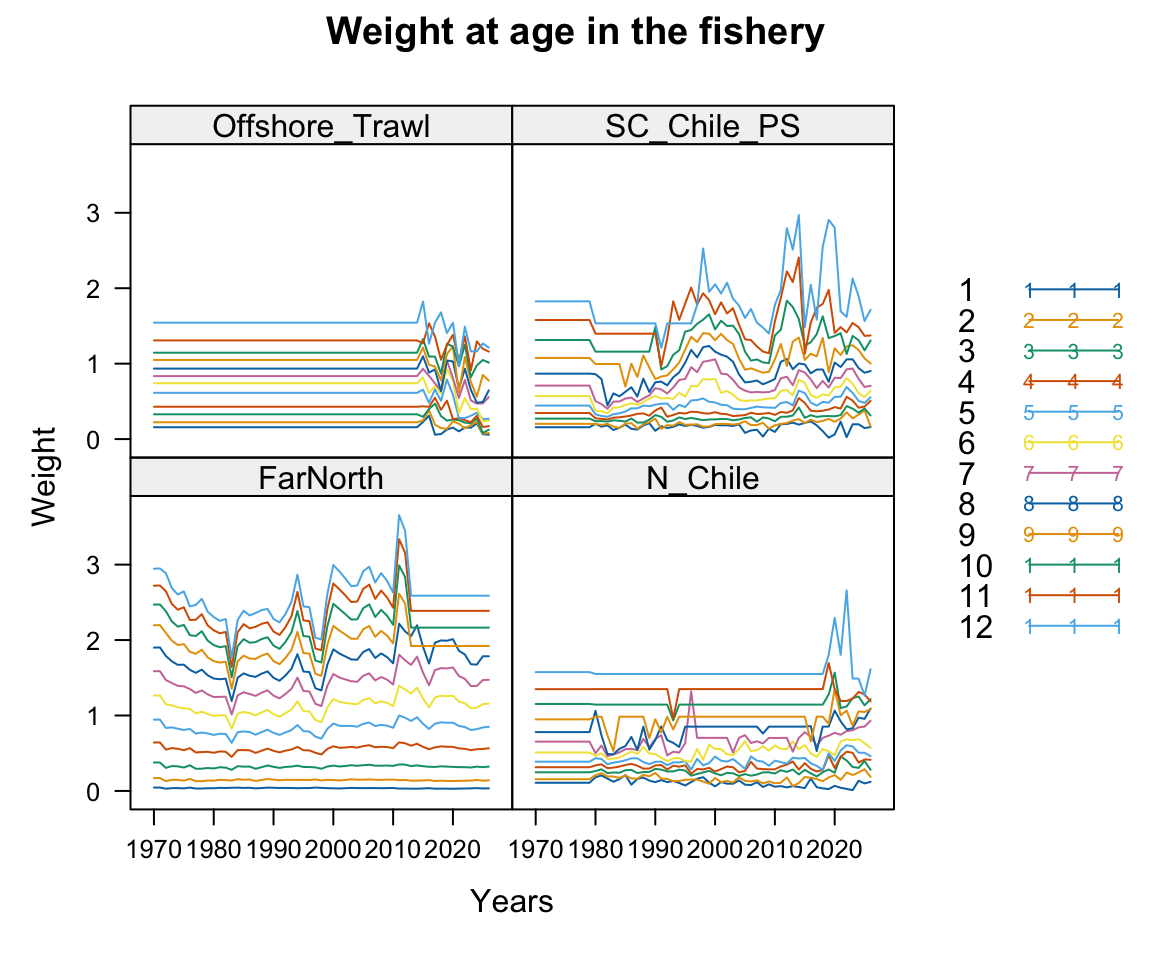
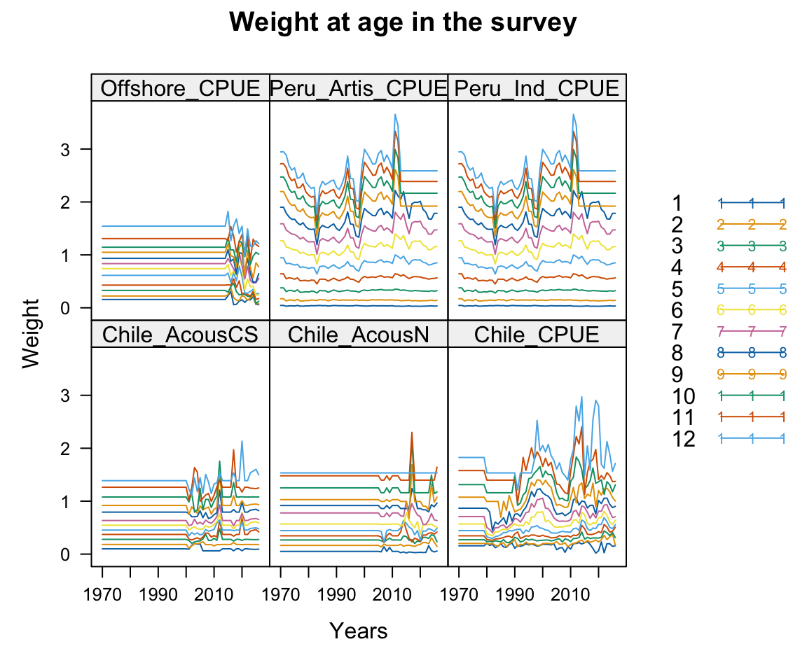
0.03 As 0.02 but with updated 2025 weight at age data for all fisheries and their associated CPUE indices
0.04 As 0.03 but replaced offshore CPUE up to 2025
0.05 As 0.04 but with 2026 catch projections
0.06 As 0.05 but with updated 2026 fishery age composition data for N_Chile, SC_Chile, and Offshore_Trawl, and updated 2026 fishery length composition data for FarNorth
0.07 As 0.06 but with updated 2026 weight at age data for N_Chile, SC_Chile, and FarNorth fleets, and for their associated CPUE indices
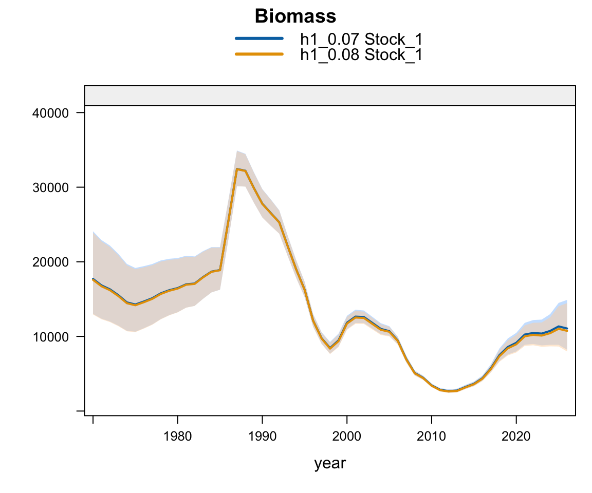
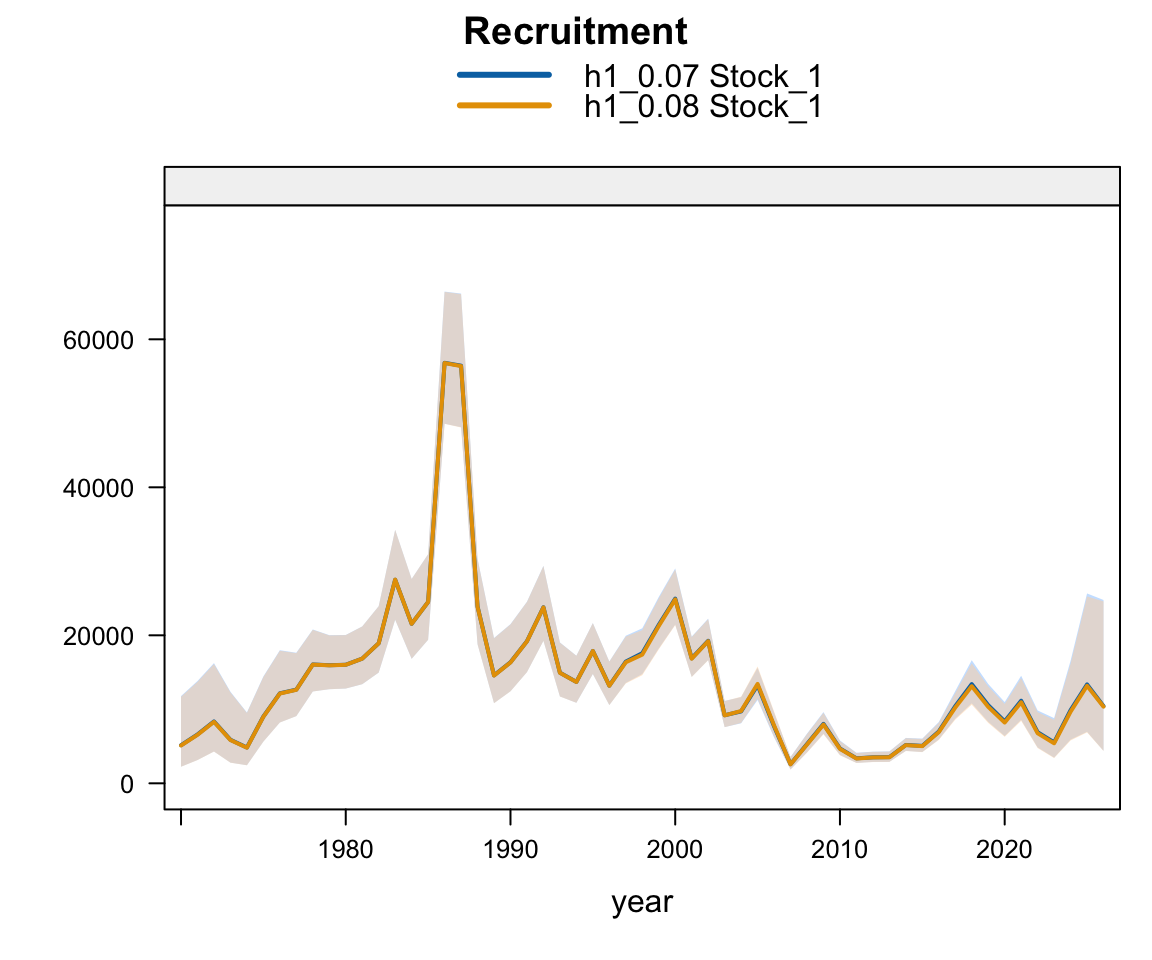
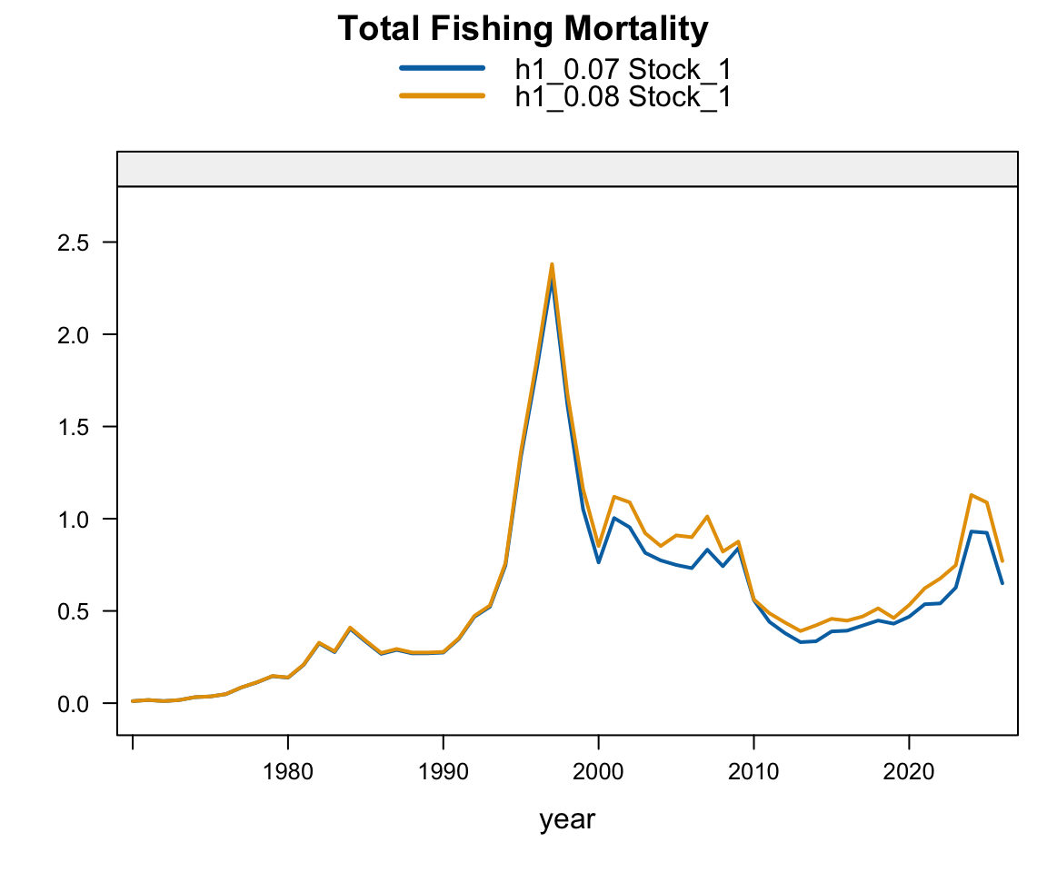
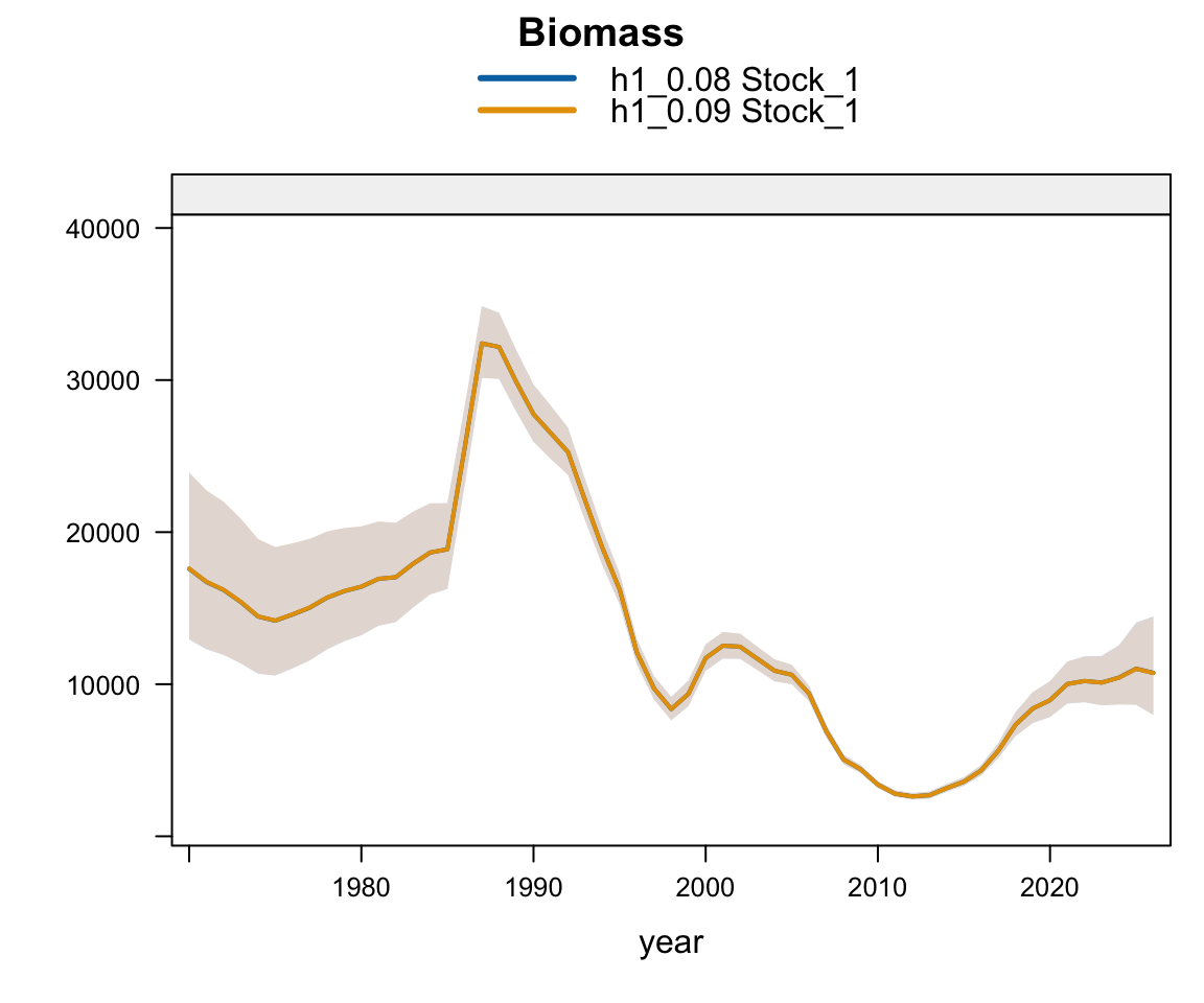
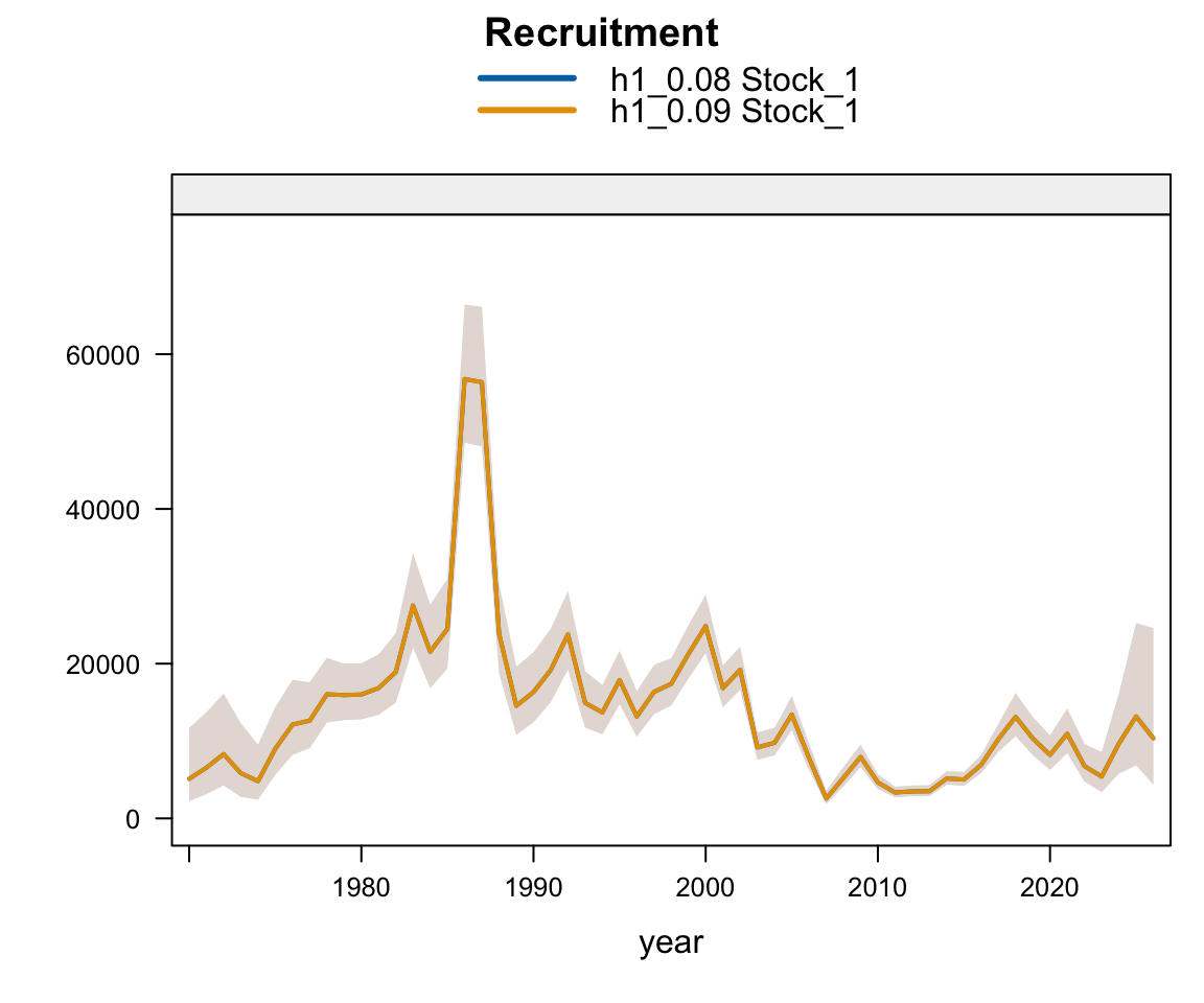
0.08 As 0.07 but replaced SC_Chile_CPUE index (updated index from SC14-JM10)
0.09 As 0.08 but replaced Peru_CPUE index
0.1 As 0.09 but updated 2026 AcousN index, with associated age composition and weight at age
Models 1.x Updated Model and Sensitivities
1 As 0.10 but with updated model (selectivity changes, recruitment) to 2026; 0.10 data file
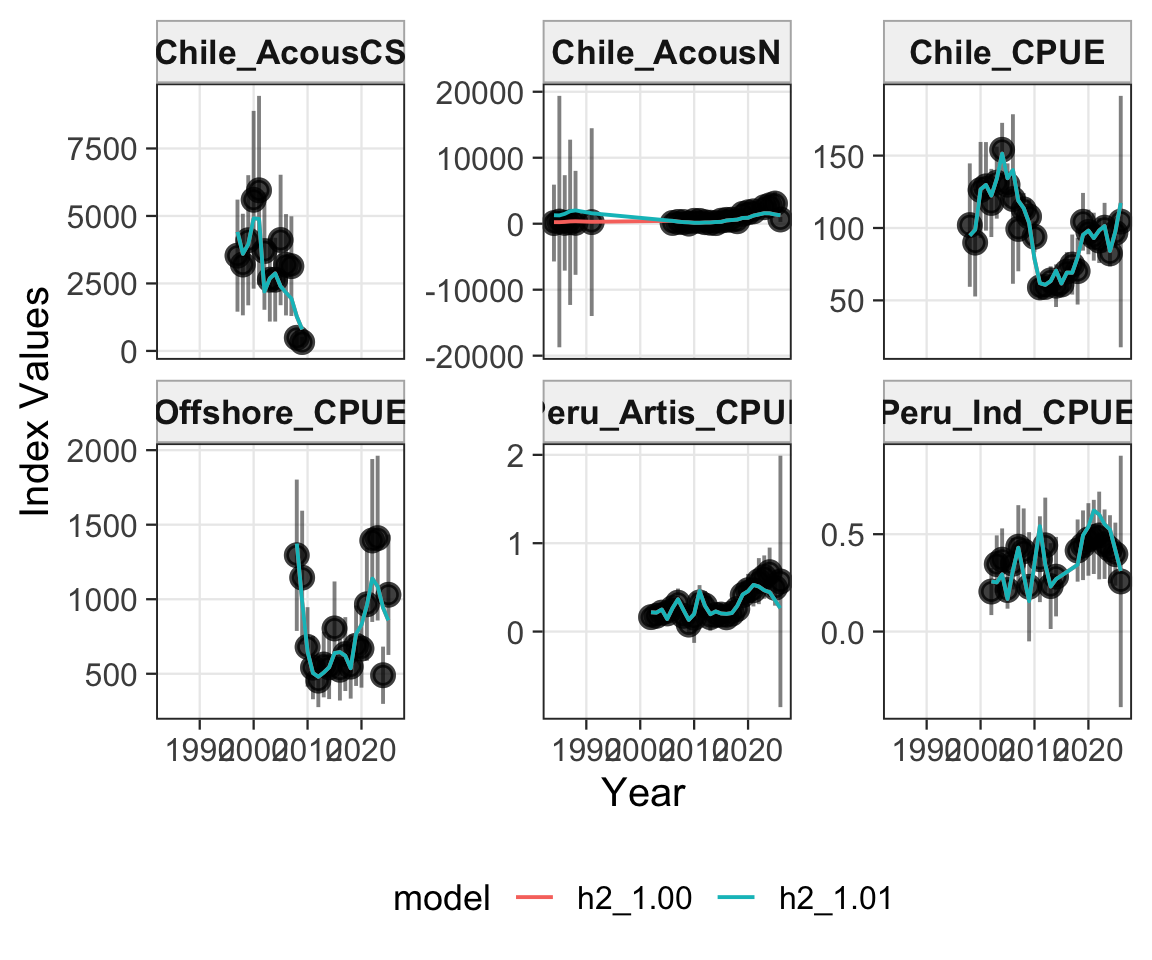
1.01 As 1.00 but removing early years (pre-2006) of Acoustic North survey data
1.02 As 1.01 but replaced SC_Chile_CPUE with one from fishing trip database (SC14-JM15)
1.03 As 1.02 but removing the 2026 data point for Chile CPUE
1.04 As 1.01 but replacing 2025/2026 weight-at-age for offshore fleet with mean across 2019-2024
1.05 As 1.04 but adding 22799 tons from Chile high seas to N_Chile fleet for 2025
1.06 As 1.05 but moving 10000 tons from FarNorth to offshore fleet for 2026
Models 1.xx.yy Base Model Projections
1.xx.ls As 1.xx but low steepness and short recruitment time series (2001-2015)

You’ll need to be in the jjm/assessment directory in order for the code here to run.

2 Re-running Last Year’s Model (a sanity check)

Re-running the 2025 model and comparing the results with that year’s SC meeting.
2.1 Single-stock hypothesis

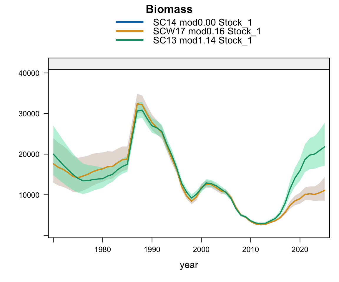
Plot comparing biomass estimated by last year’s model (mod_preBM) with the benchmark model (mod_BM) and a re-run of the model this year (h1_0.00).

Plot comparing biomass estimated by last year’s model (mod_preBM) with the benchmark model (mod_BM) and a re-run of the model this year (h1_0.00).

Plot comparing recruitment estimated by last year’s model (mod_preBM) with the benchmark model (mod_BM) and a re-run of the model this year (h1_0.00).

Plot comparing recruitment estimated by last year’s model (mod_preBM) with the benchmark model (mod_BM) and a re-run of the model this year (h1_0.00).

Plot comparing fishing mortality estimated by last year’s model (mod_preBM) with the benchmark model (mod_BM) and a re-run of the model this year (h1_0.00).

Plot comparing fishing mortality estimated by last year’s model (mod_preBM) with the benchmark model (mod_BM) and a re-run of the model this year (h1_0.00).

2.2 Two-stock hypothesis

Plot comparing biomass estimated by last year’s model (mod_preBM) with the benchmark model (mod_prev) and a re-run of the model this year (h2_0.00).

Plot comparing biomass estimated by last year’s model (mod_preBM) with the benchmark model (mod_prev) and a re-run of the model this year (h2_0.00).

Plot comparing recruitment estimated by last year’s model (mod_preBM) with the benchmark model (mod_prev) and a re-run of the model this year (h2_0.00).

Plot comparing recruitment estimated by last year’s model (mod_preBM) with the benchmark model (mod_prev) and a re-run of the model this year (h2_0.00).

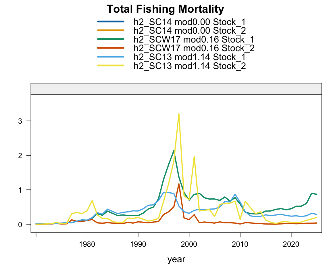
Plot comparing fishing mortality estimated by last year’s model (mod_preBM) with the benchmark model (mod_prev) and a re-run of the model this year (h2_0.00).

Plot comparing fishing mortality estimated by last year’s model (mod_preBM) with the benchmark model (mod_prev) and a re-run of the model this year (h2_0.00).

3 Updated Data

3.1 Datasets

4 Incremental Data Updates

The most updated table of model runs can be found on Github.

4.1 Updating last year’s data

The data updated to 2025, includes catch estimates, age and length compositions, and indices of abundance.
4.1.1 Single-stock hypothesis

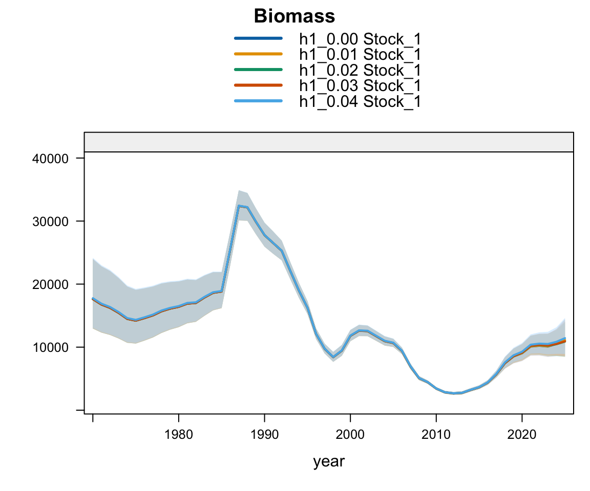
Plot comparing biomass estimated by last year’s model (h1_0.00) with data updated to 2025.

Plot comparing biomass estimated by last year’s model (h1_0.00) with data updated to 2025.

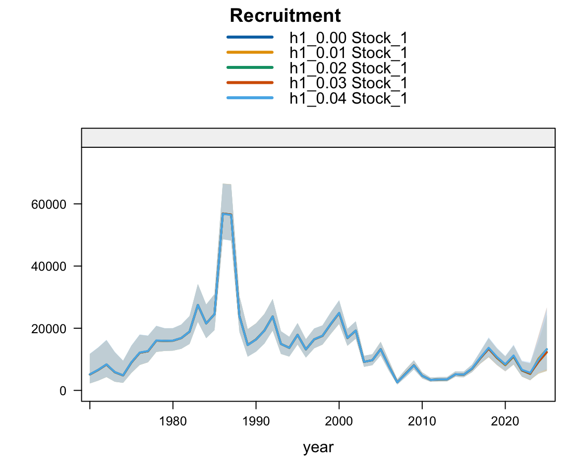
Plot comparing recruitment estimated by last year’s model (h1_0.00) with data updated to 2025.

Plot comparing recruitment estimated by last year’s model (h1_0.00) with data updated to 2025.

Plot comparing fishing mortality estimated by last year’s model (h1_0.00) with data updated to 2025.

Plot comparing fishing mortality estimated by last year’s model (h1_0.00) with data updated to 2025.

4.1.2 Two-stock hypothesis

Plot comparing biomass estimated by last year’s model (h2_0.00) with data updated to 2025.

Plot comparing biomass estimated by last year’s model (h2_0.00) with data updated to 2025.

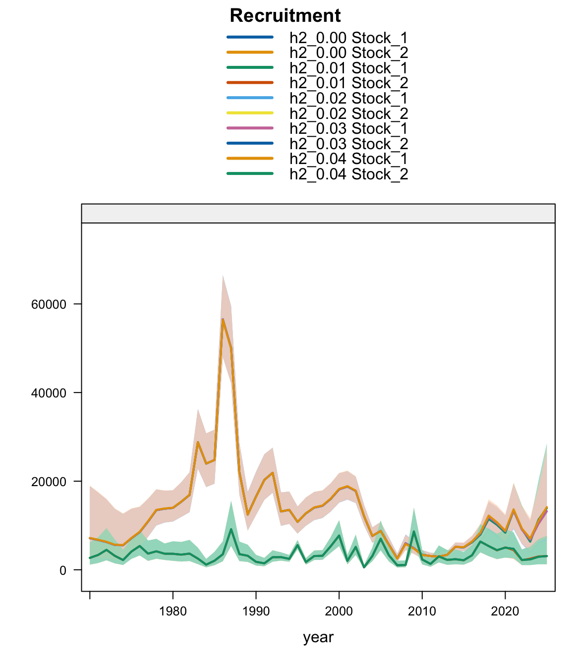
Plot comparing recruitment estimated by last year’s model (h2_0.00) with data updated to 2025.

Plot comparing recruitment estimated by last year’s model (h2_0.00) with data updated to 2025.

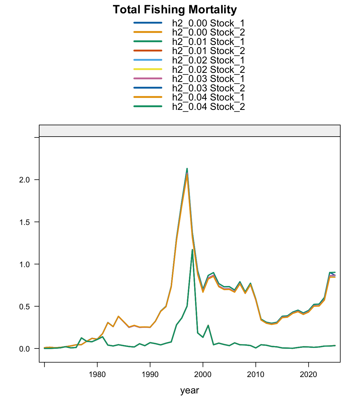
Plot comparing fishing mortality estimated by last year’s model (h2_0.00) with data updated to 2025.

Plot comparing fishing mortality estimated by last year’s model (h2_0.00) with data updated to 2025.

4.2 Updating this year’s data

The data updated to 2026 include projected catch estimates, age and length compositions, and indices of abundance.
4.2.1 Single-stock hypothesis

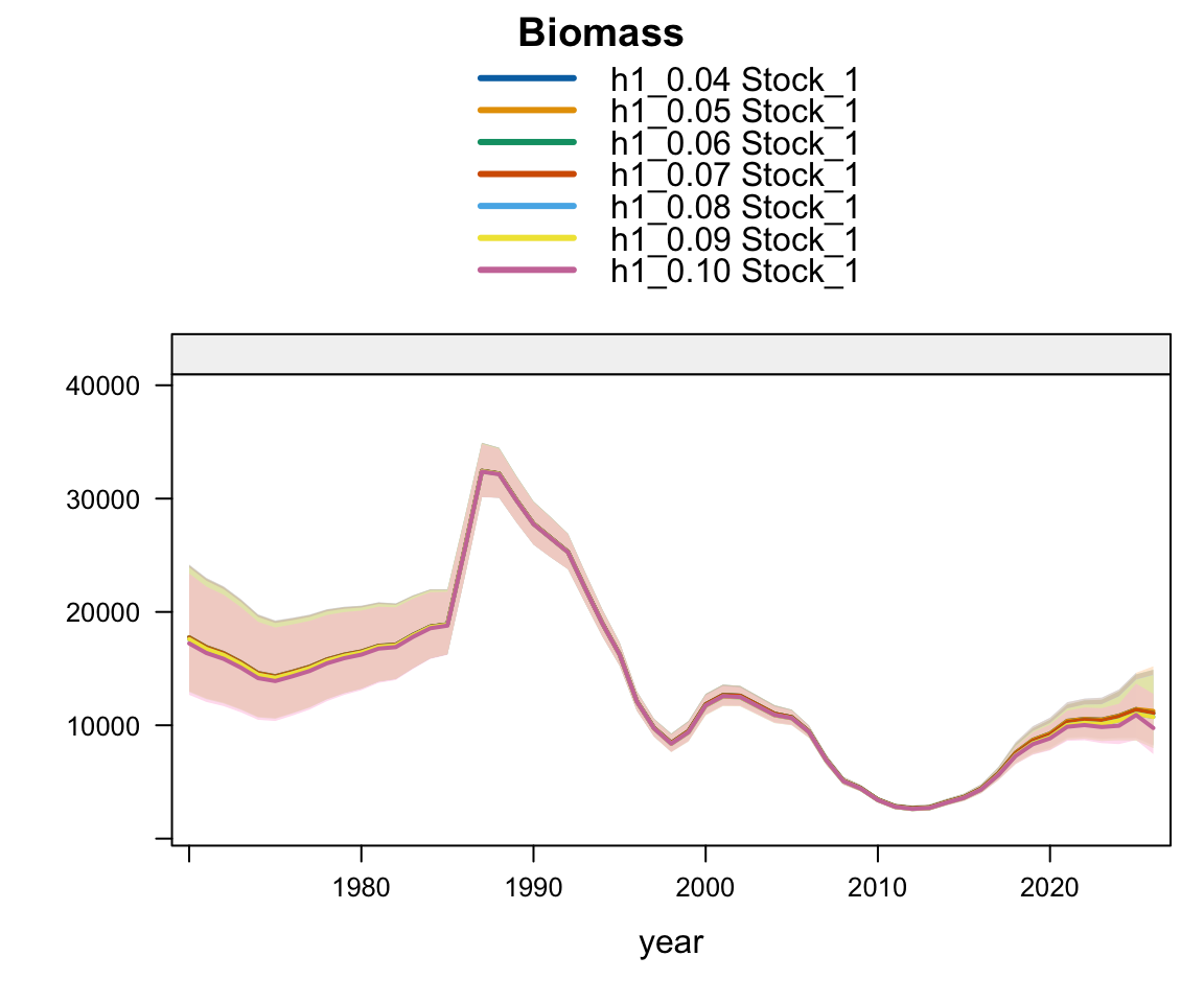
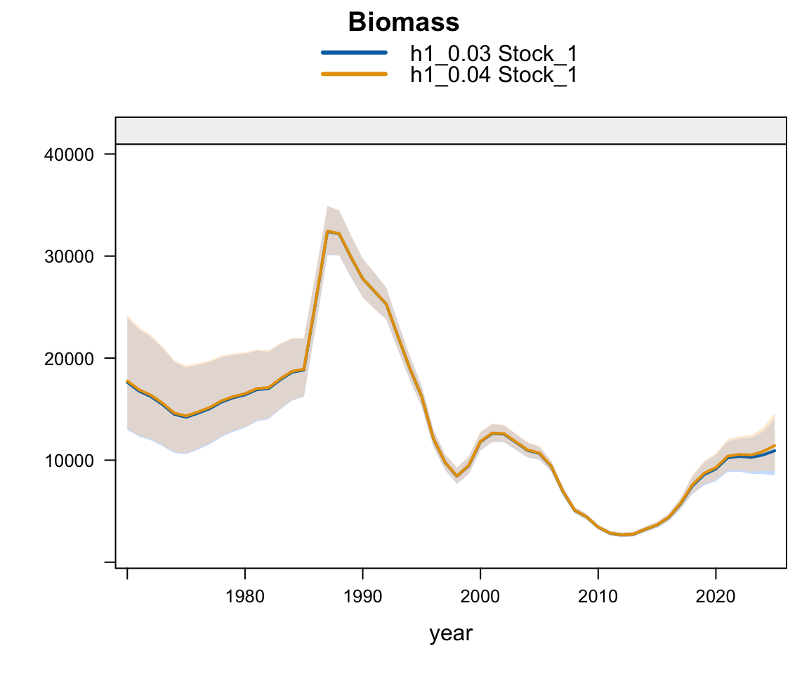
Plot comparing biomass estimated with last year’s data using the same model (h1_0.04) but with data updated to 2026.

Plot comparing biomass estimated with last year’s data using the same model (h1_0.04) but with data updated to 2026.

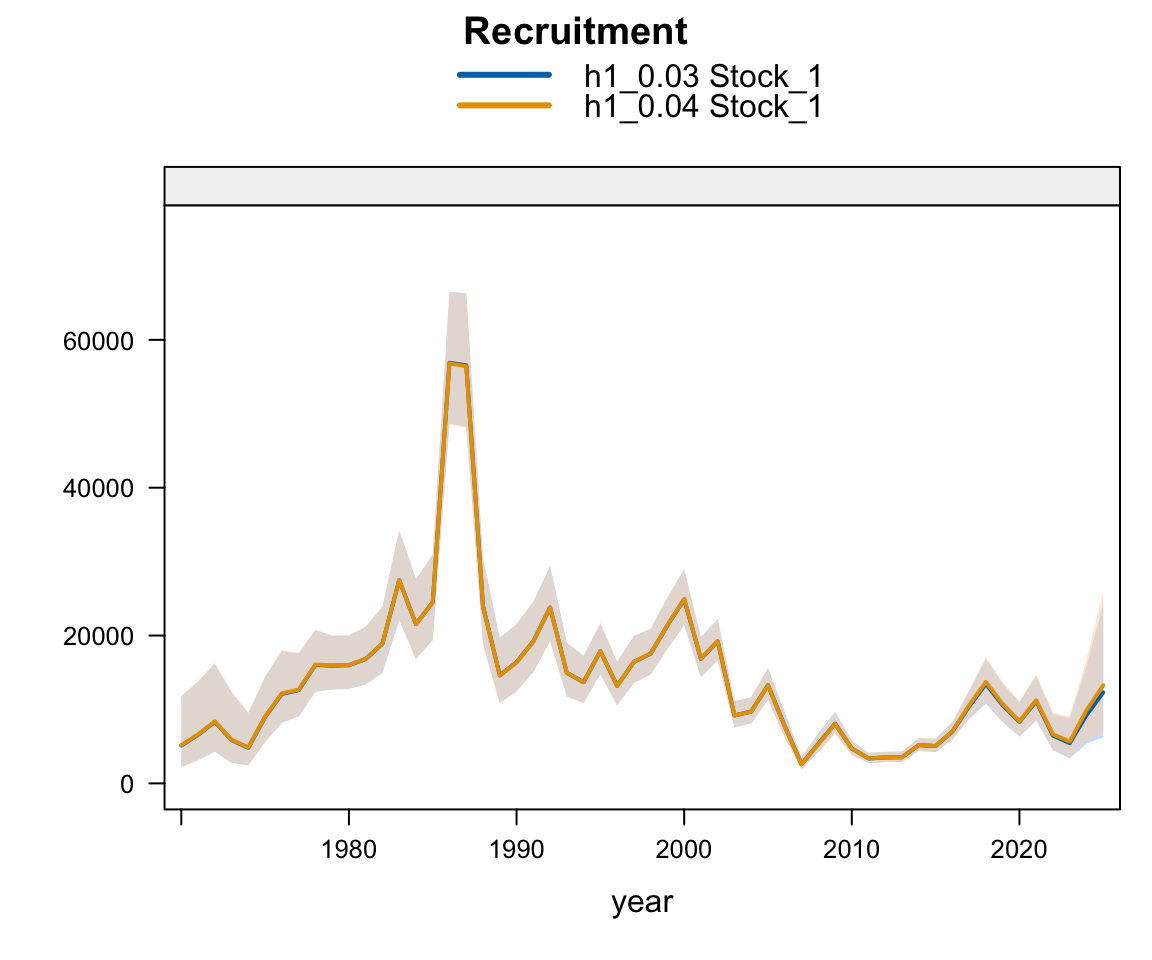
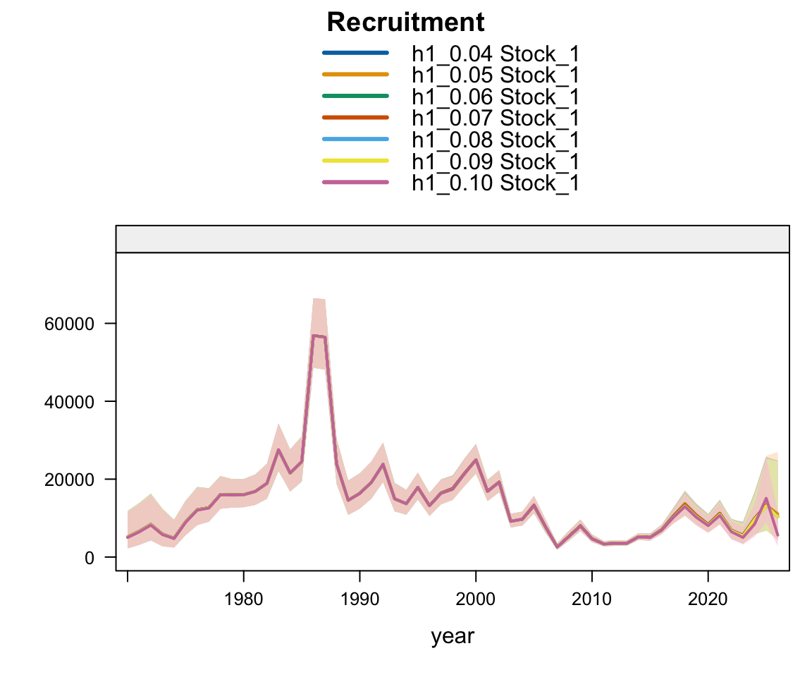
Plot comparing recruitment estimated with last year’s data using the same model (h1_0.04) but with data updated to 2026.

Plot comparing recruitment estimated with last year’s data using the same model (h1_0.04) but with data updated to 2026.

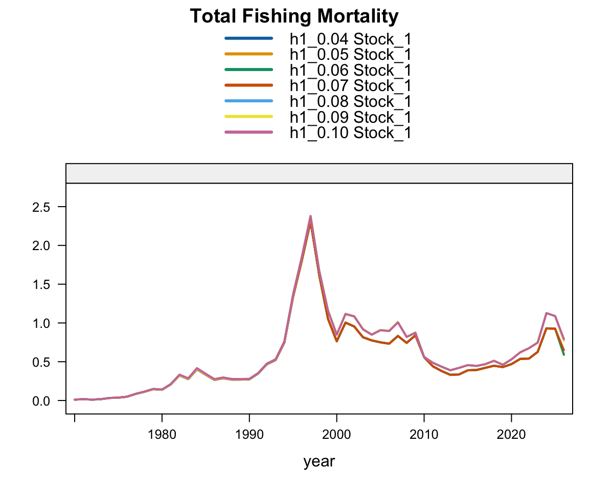
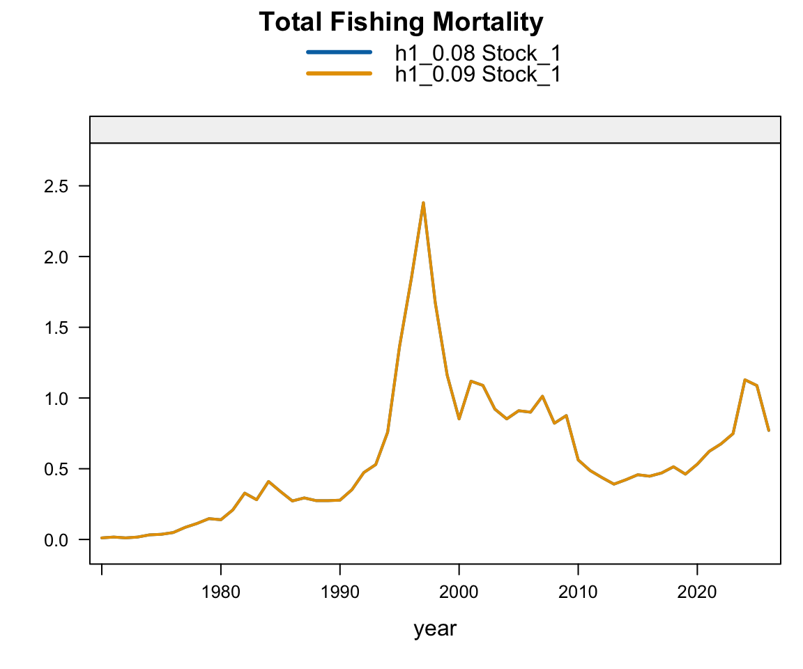
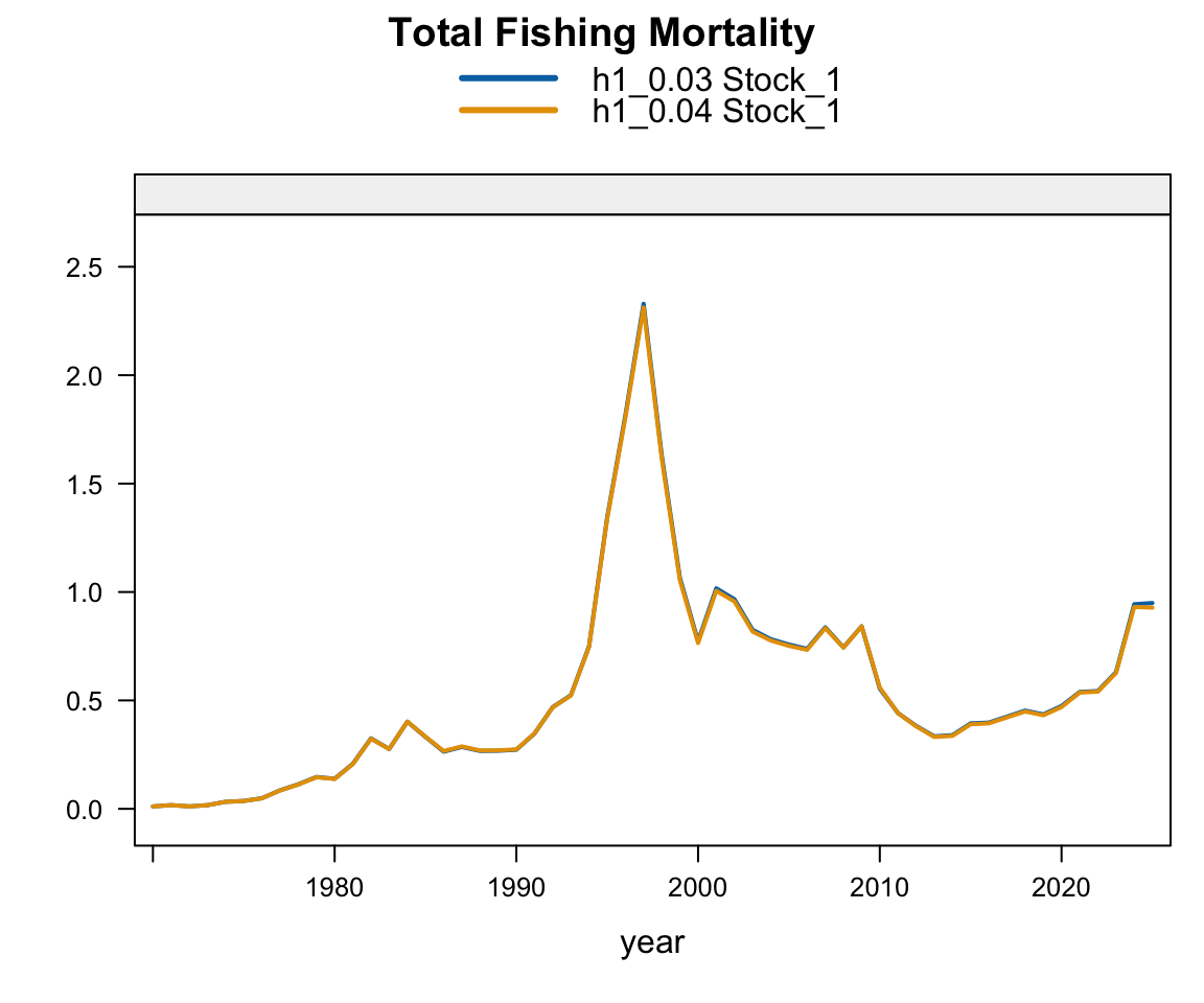
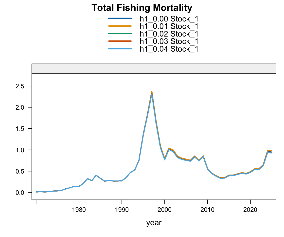
Plot comparing fishing mortality estimated with last year’s data using the same model (h1_0.04) but with data updated to 2026.

Plot comparing fishing mortality estimated with last year’s data using the same model (h1_0.04) but with data updated to 2026.

4.2.2 Two-stock hypothesis

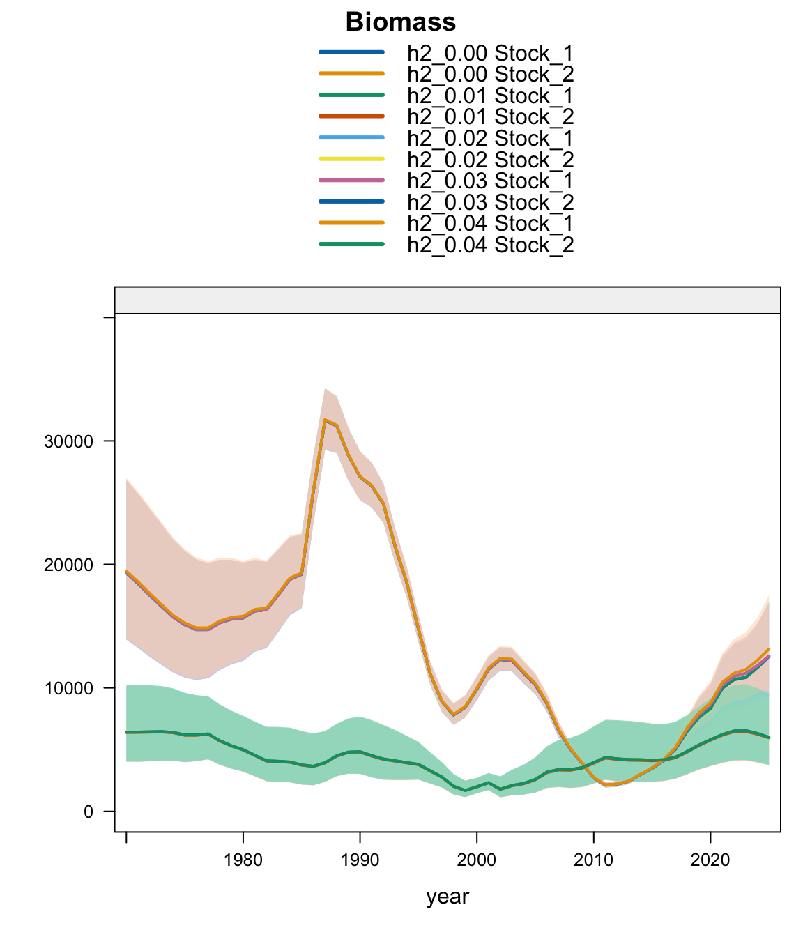
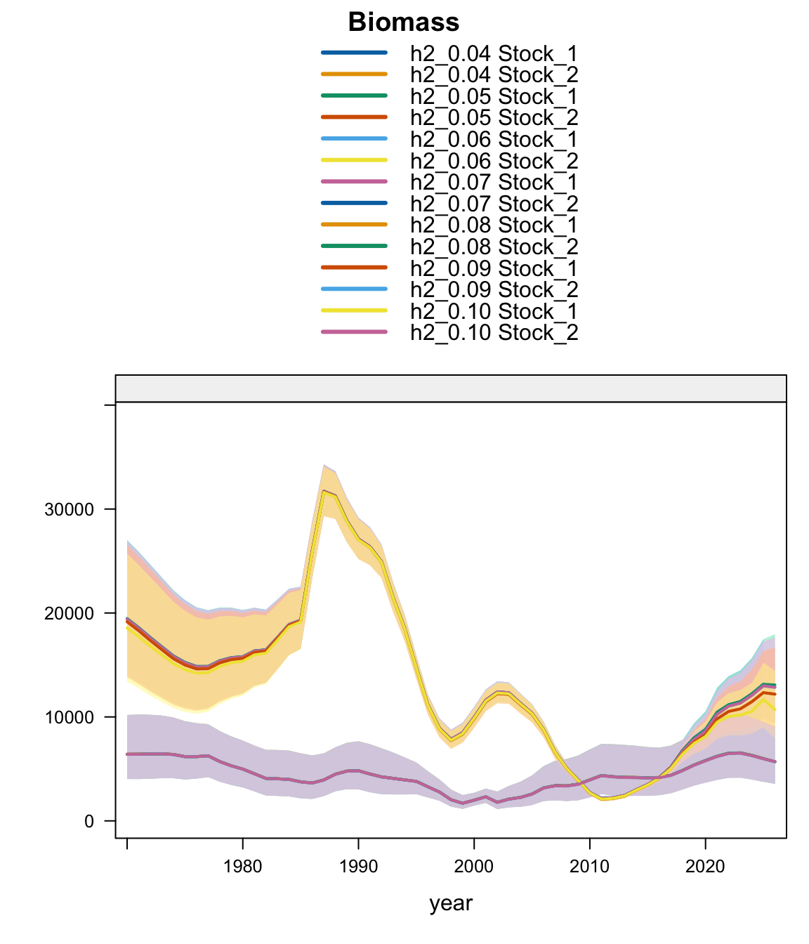
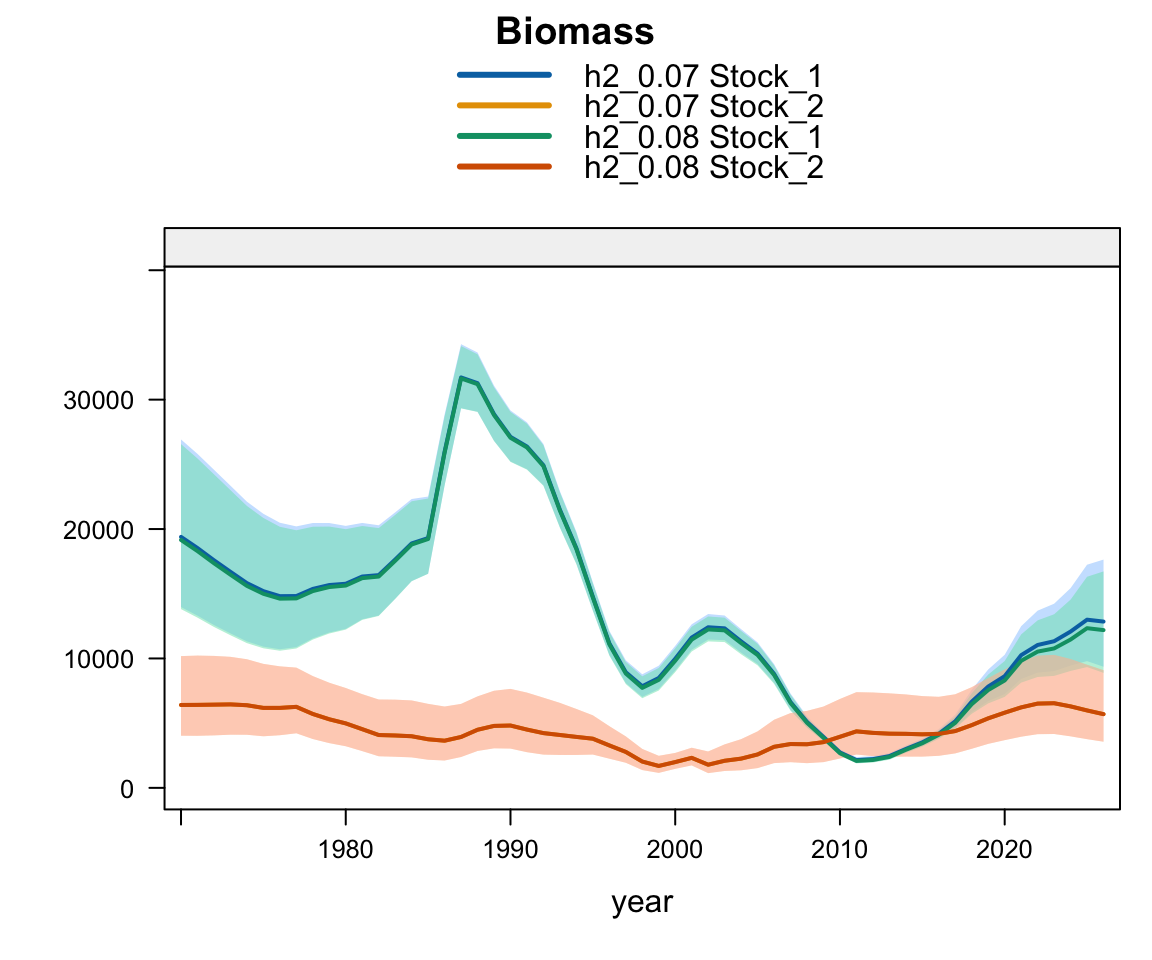
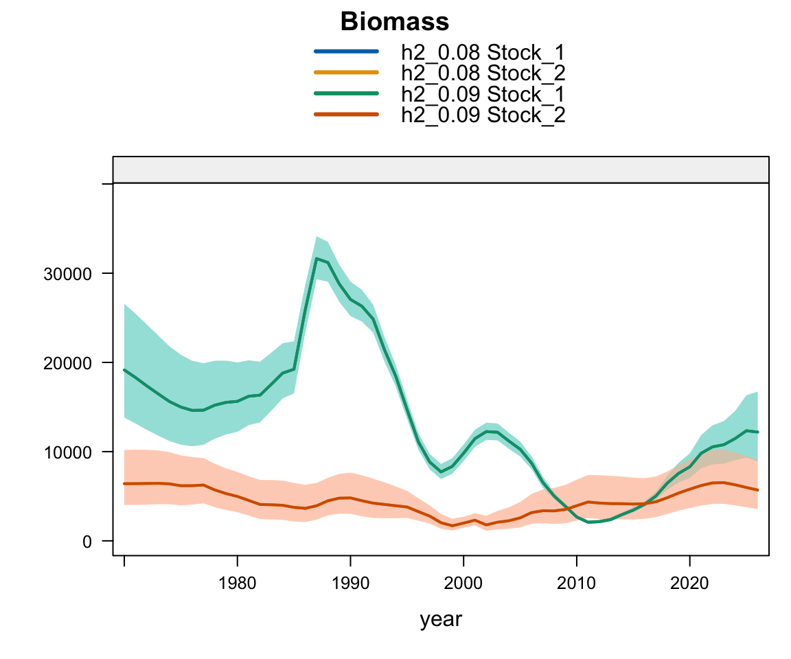
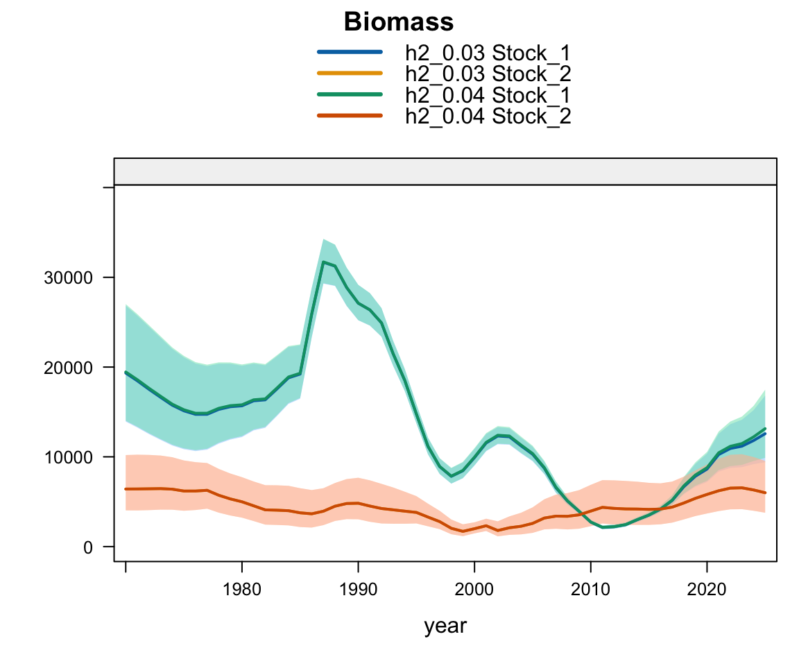
Plot comparing biomass estimated with last year’s data using the same model (h2_0.04) but with data updated to 2026.

Plot comparing biomass estimated with last year’s data using the same model (h2_0.04) but with data updated to 2026.

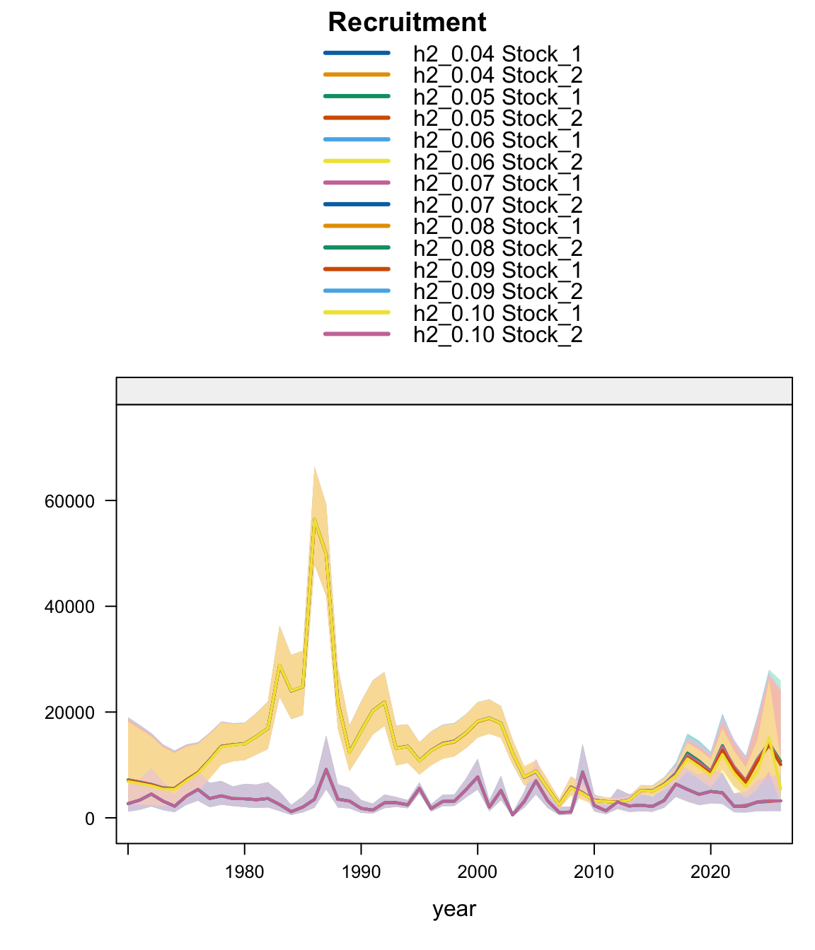
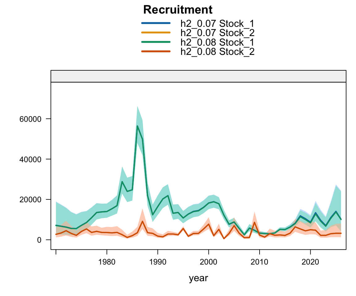
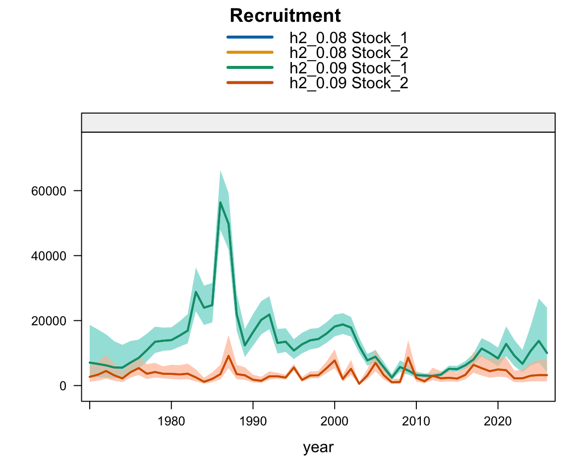
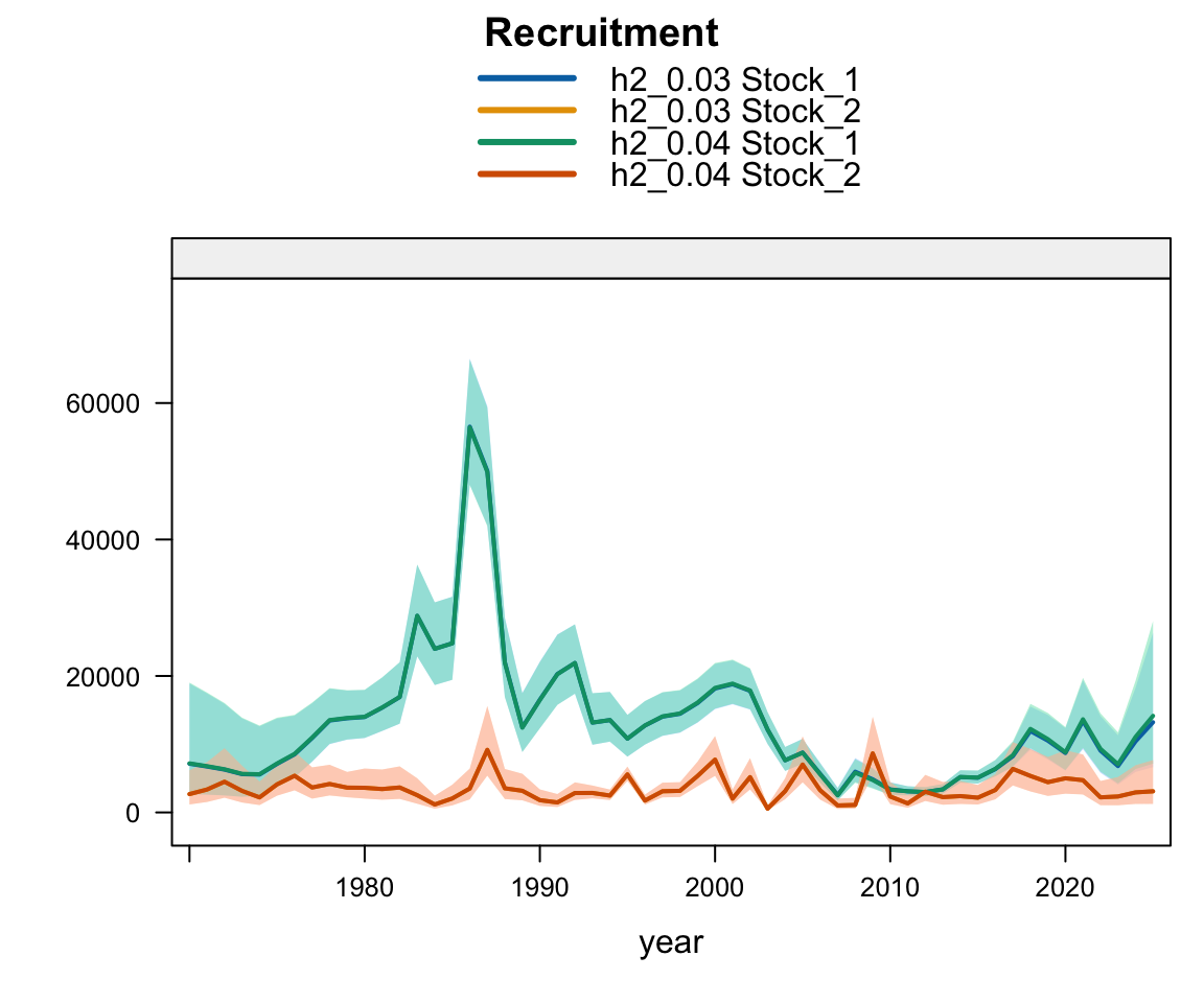
Plot comparing recruitment estimated with last year’s data using the same model (h2_0.04) but with data updated to 2026.

Plot comparing recruitment estimated with last year’s data using the same model (h2_0.04) but with data updated to 2026.

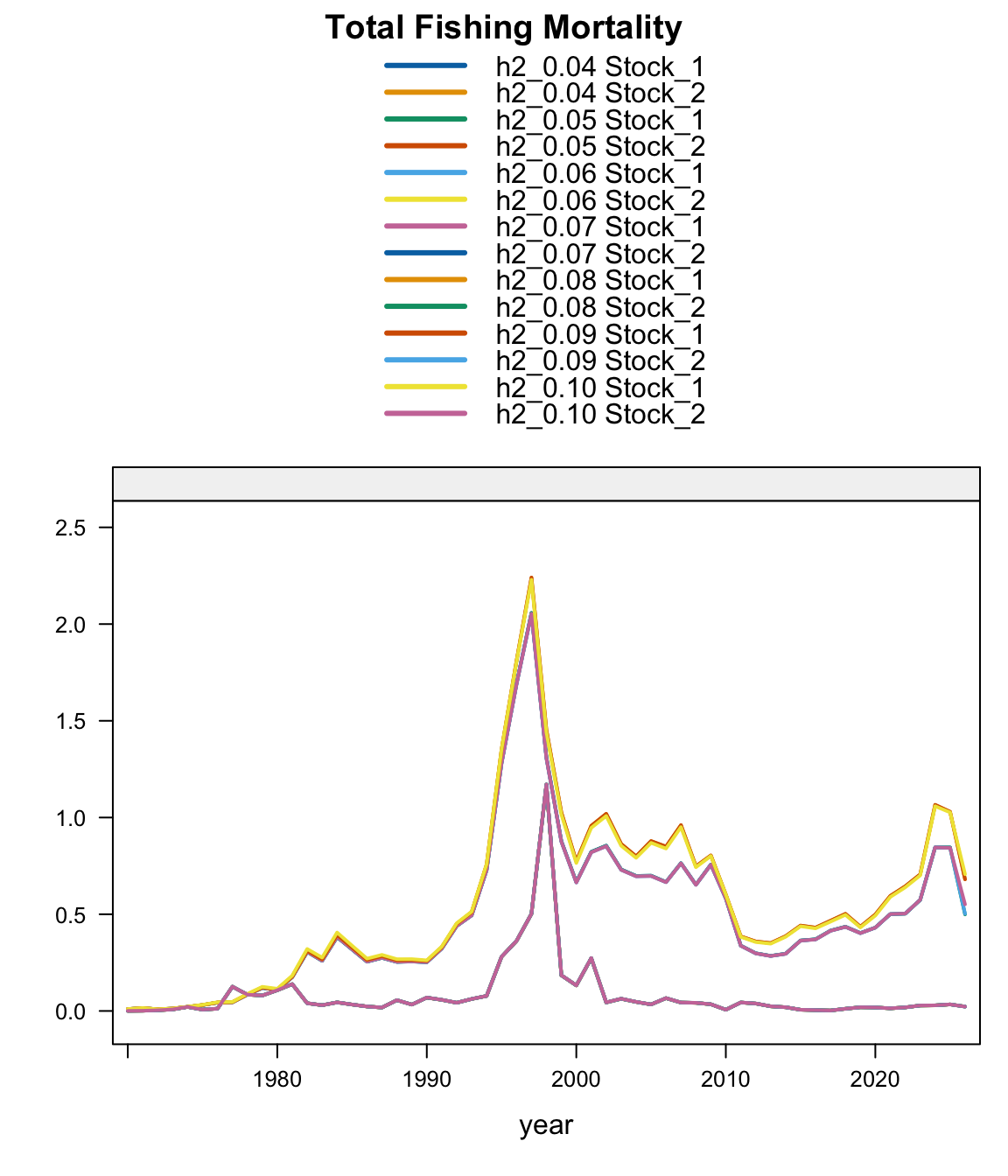
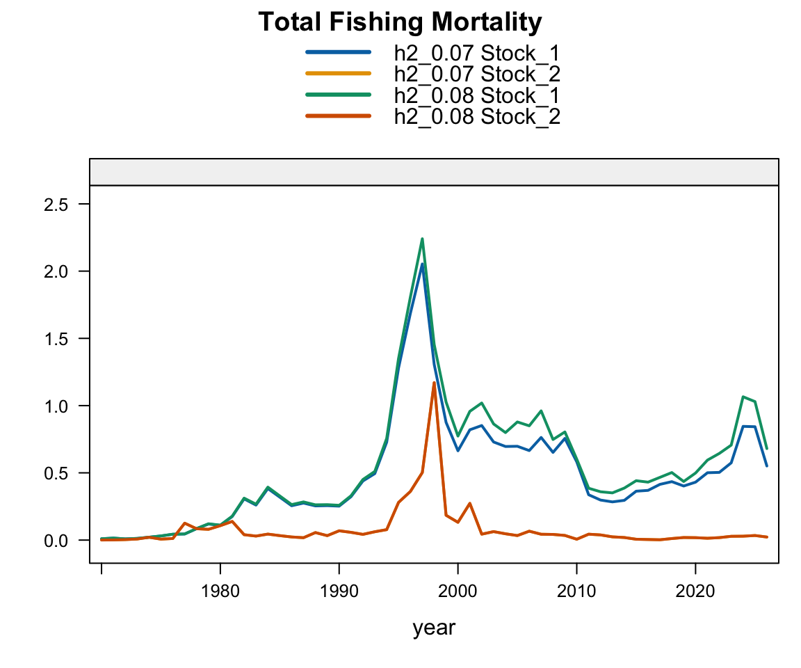
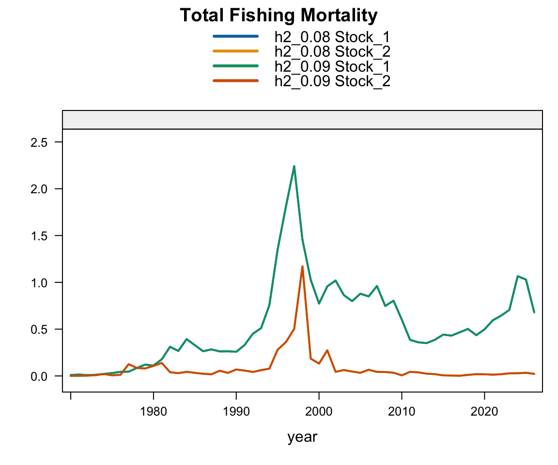
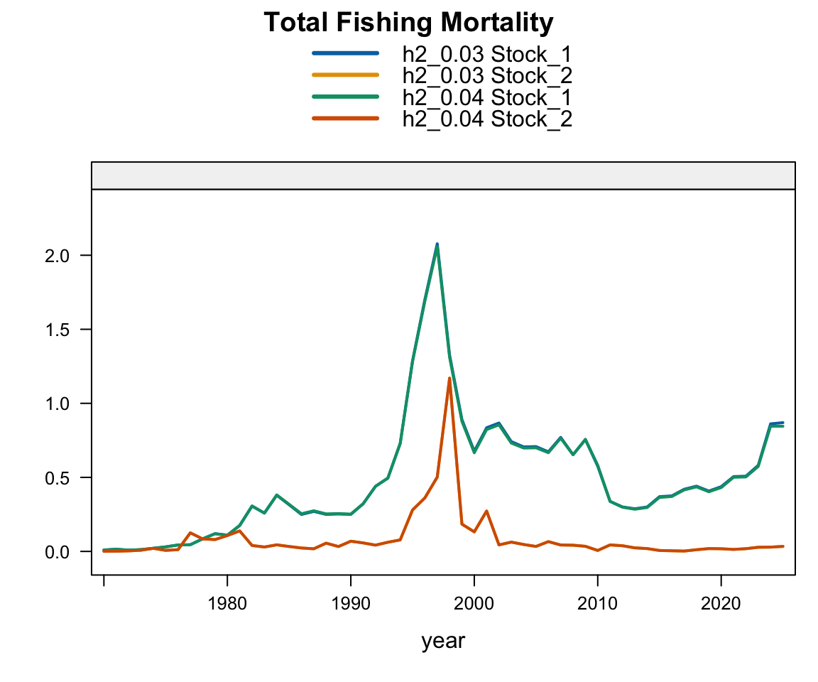
Plot comparing fishing mortality estimated with last year’s data using the same model (h2_0.04) but with data updated to 2026.

Plot comparing fishing mortality estimated with last year’s data using the same model (h2_0.04) but with data updated to 2026.

4.3 Stepping through the CPUE replacements

4.3.1 SC Chile CPUE

4.3.1.1 Single-stock hypothesis

4.3.1.2 Two-stock hypothesis

4.3.2 Peru CPUE

4.3.2.1 Comparison of the index from previous years

4.3.2.2 Single-stock hypothesis

4.3.2.3 Two-stock hypothesis

4.3.3 Offshore CPUE

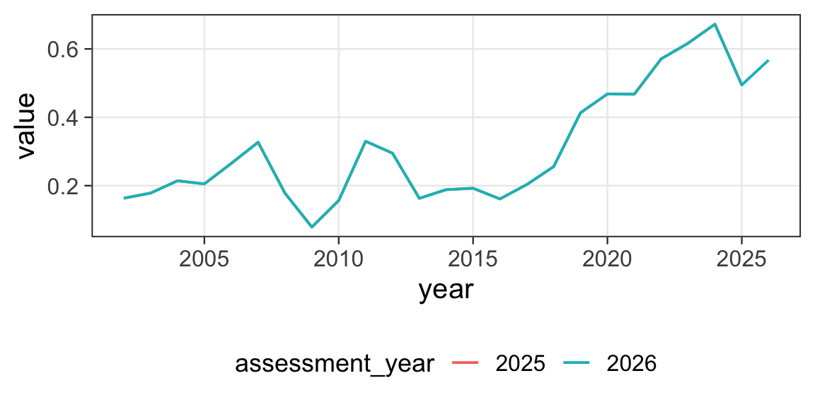
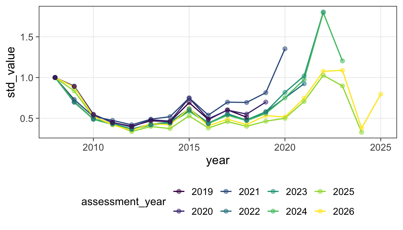
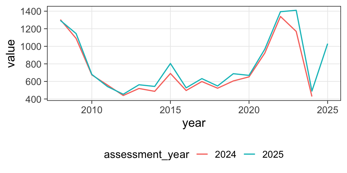
Note that this time series ends in 2025.
4.3.3.1 Comparison of the index from previous years

4.3.3.2 Single-stock hypothesis

4.3.3.3 Two-stock hypothesis

5 Final Data Update

This shows the final data update, using the exact same model (i.e., with the same control files).
5.1 Single-stock hypothesis

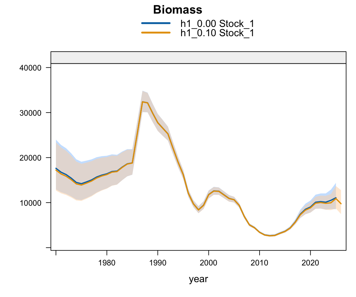
Plot comparing biomass estimated by last year’s model (h1_0.00) with data updated to 2026 (h1_0.10).

Plot comparing biomass estimated by last year’s model (h1_0.00) with data updated to 2026 (h1_0.10).

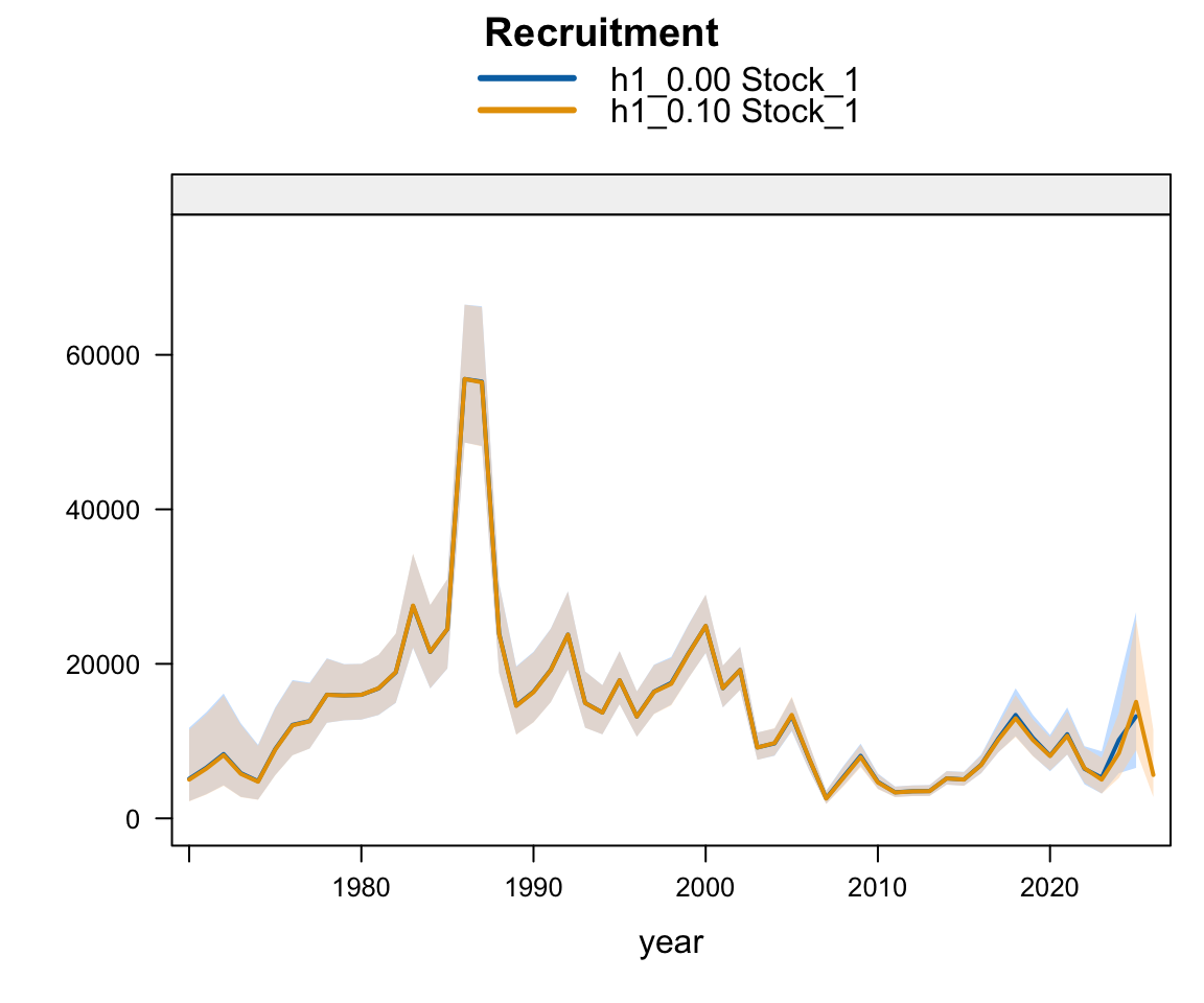
Plot comparing recruitment estimated by last year’s model (h1_0.00) with data updated to 2026 (h1_0.10).

Plot comparing recruitment estimated by last year’s model (h1_0.00) with data updated to 2026 (h1_0.10).

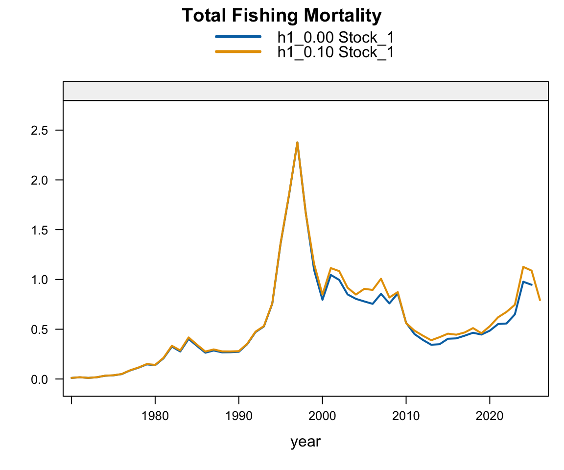
Plot comparing fishing mortality estimated by last year’s model (h1_0.00) with data updated to 2026 (h1_0.10).

Plot comparing fishing mortality estimated by last year’s model (h1_0.00) with data updated to 2026 (h1_0.10).

5.2 Two-stock hypothesis

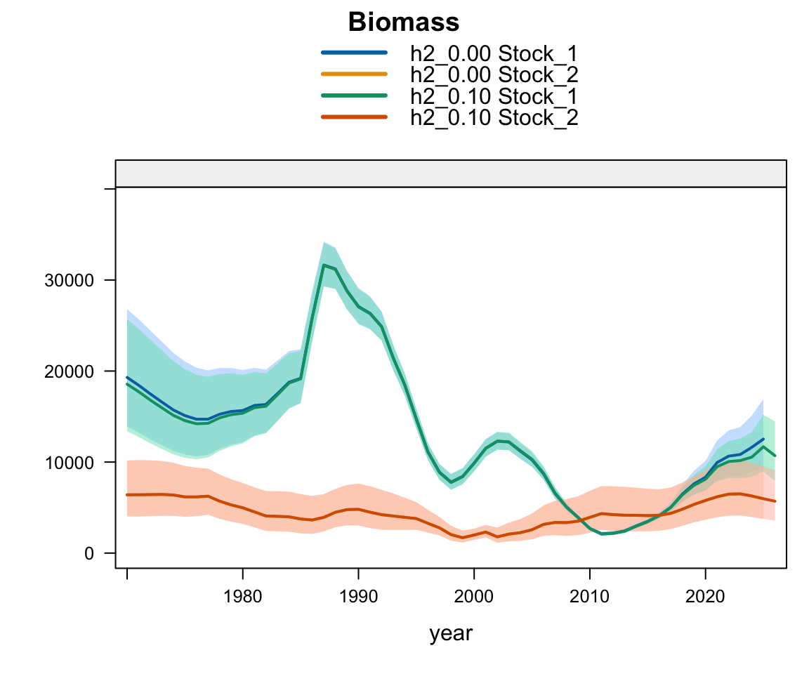
Plot comparing fishing mortality estimated by last year’s model (h2_0.00) with data updated to 2026 (h2_0.10).

Plot comparing fishing mortality estimated by last year’s model (h2_0.00) with data updated to 2026 (h2_0.10).

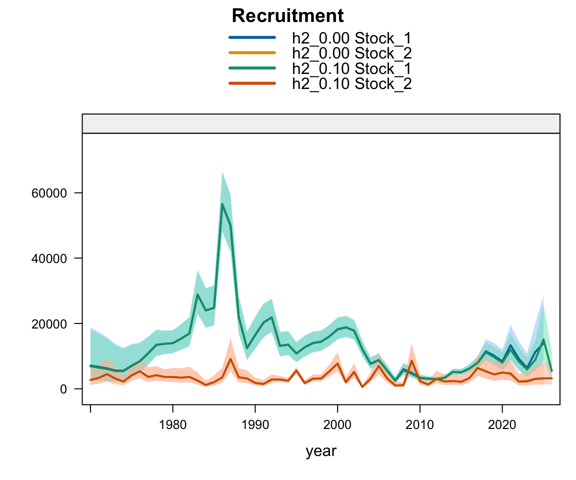
Plot comparing recruitment estimated by last year’s model (h2_0.00) with data updated to 2026 (h2_0.10).

Plot comparing recruitment estimated by last year’s model (h2_0.00) with data updated to 2026 (h2_0.10).

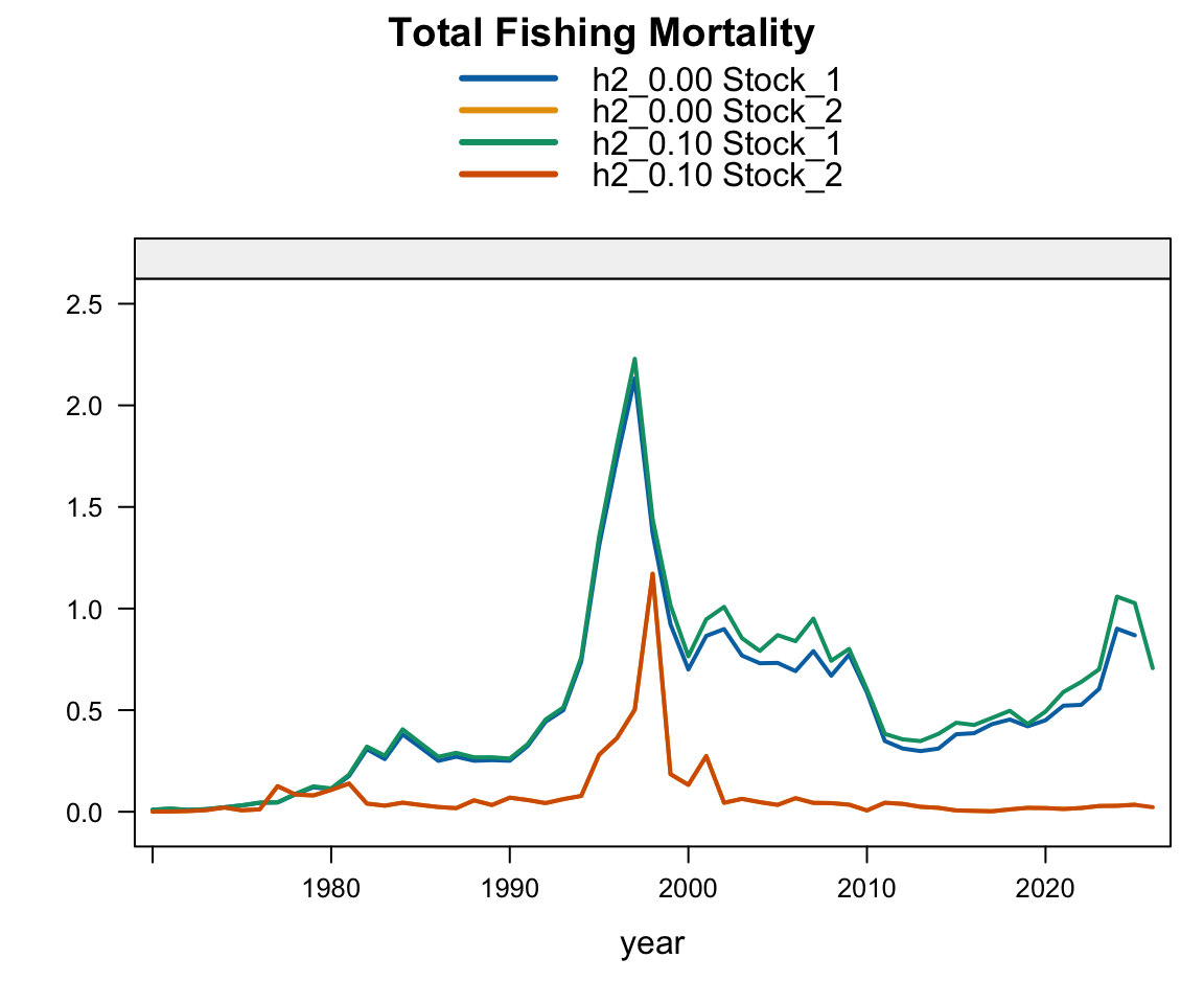
Plot comparing fishing mortality estimated by last year’s model (h2_0.00) with data updated to 2026 (h2_0.10).

Plot comparing fishing mortality estimated by last year’s model (h2_0.00) with data updated to 2026 (h2_0.10).

6 Model Update

These results are from updating the model to include selectivity changes in the most recent year, and to extend the recruitment regime shift time series. This is the same procedure that was applied in previous years.
6.1 Single-stock hypothesis

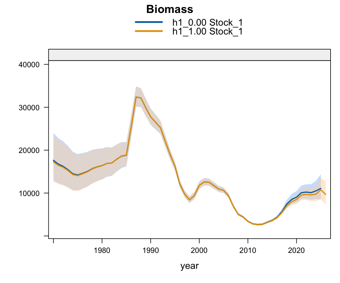
Plot comparing biomass estimates from last year’s model (h1_0.00) to this year’s (h1_1.00).

Plot comparing biomass estimates from last year’s model (h1_0.00) to this year’s (h1_1.00).

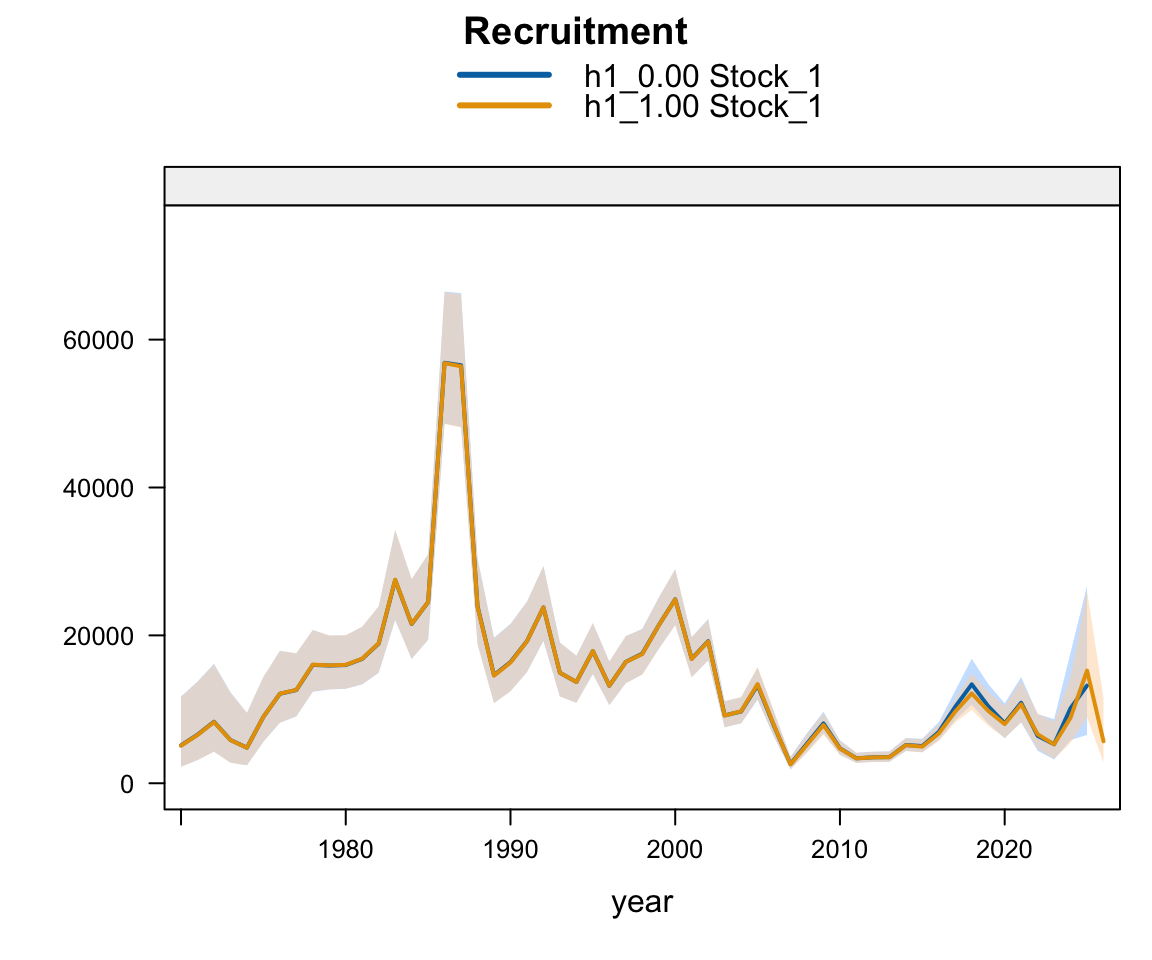
Plot comparing recruitment estimates from last year’s model (h1_0.00) to this year’s (h1_1.00).

Plot comparing recruitment estimates from last year’s model (h1_0.00) to this year’s (h1_1.00).

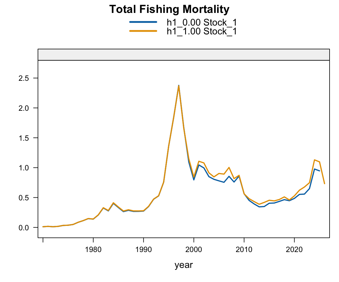
Plot comparing fishing mortality estimates from last year’s model (h1_0.00) to this year’s (h1_1.00).

Plot comparing fishing mortality estimates from last year’s model (h1_0.00) to this year’s (h1_1.00).

6.2 Two-stock hypothesis

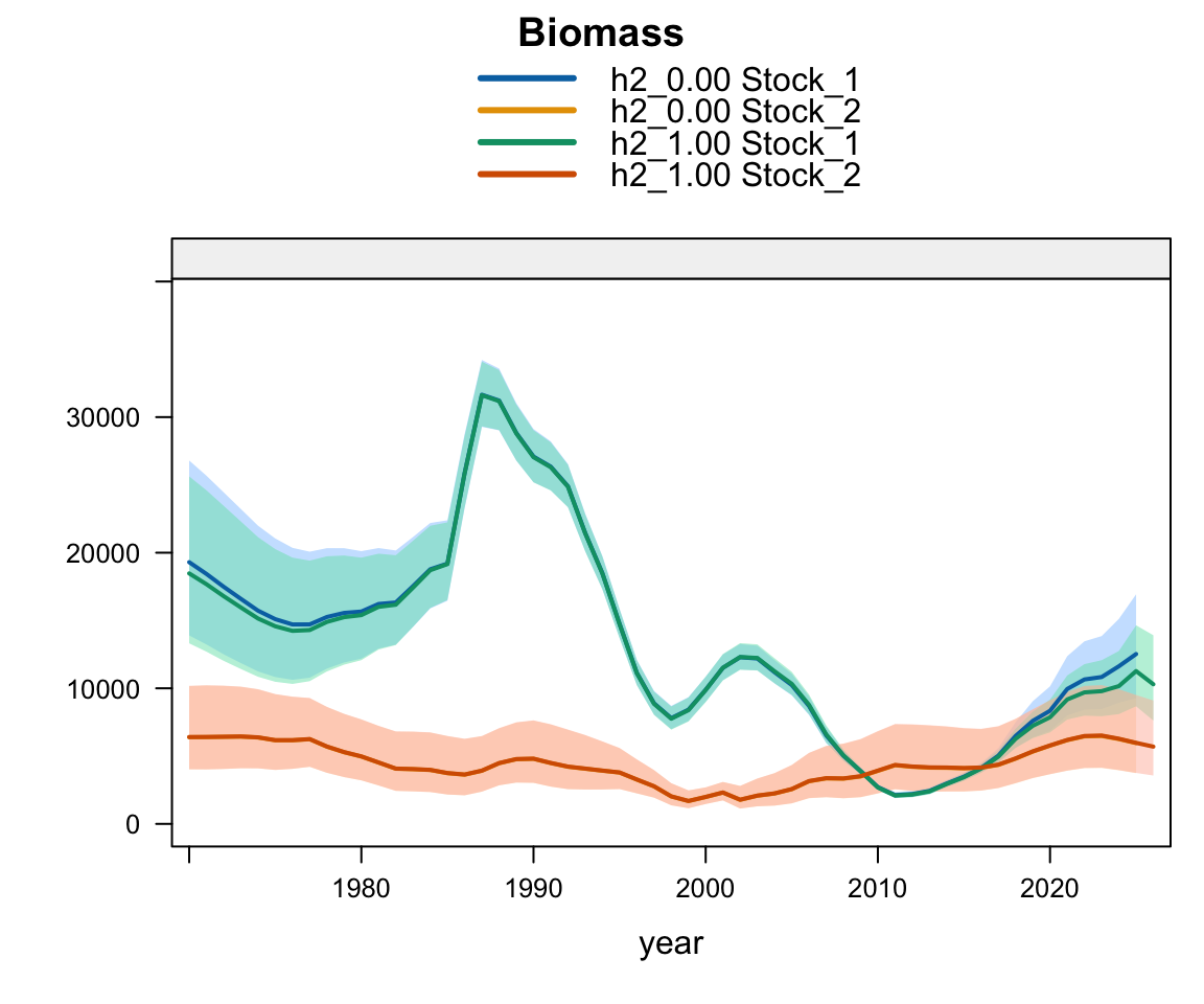
Plot comparing biomass estimated by last year’s model (h2_0.00) to this year’s (h2_1.00).

Plot comparing biomass estimated by last year’s model (h2_0.00) to this year’s (h2_1.00).

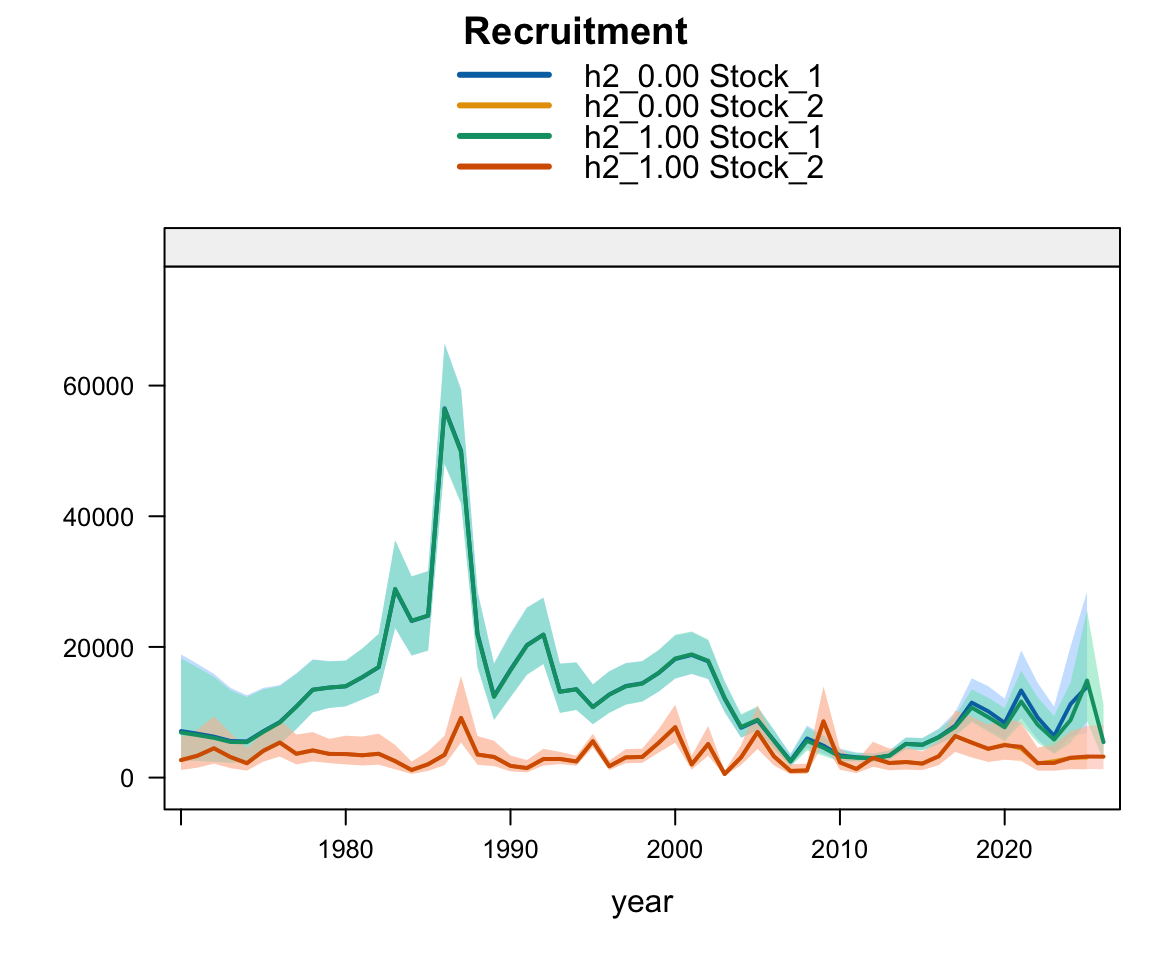
Plot comparing recruitment estimated by last year’s model (h2_0.00) to this year’s (h2_1.00).

Plot comparing recruitment estimated by last year’s model (h2_0.00) to this year’s (h2_1.00).

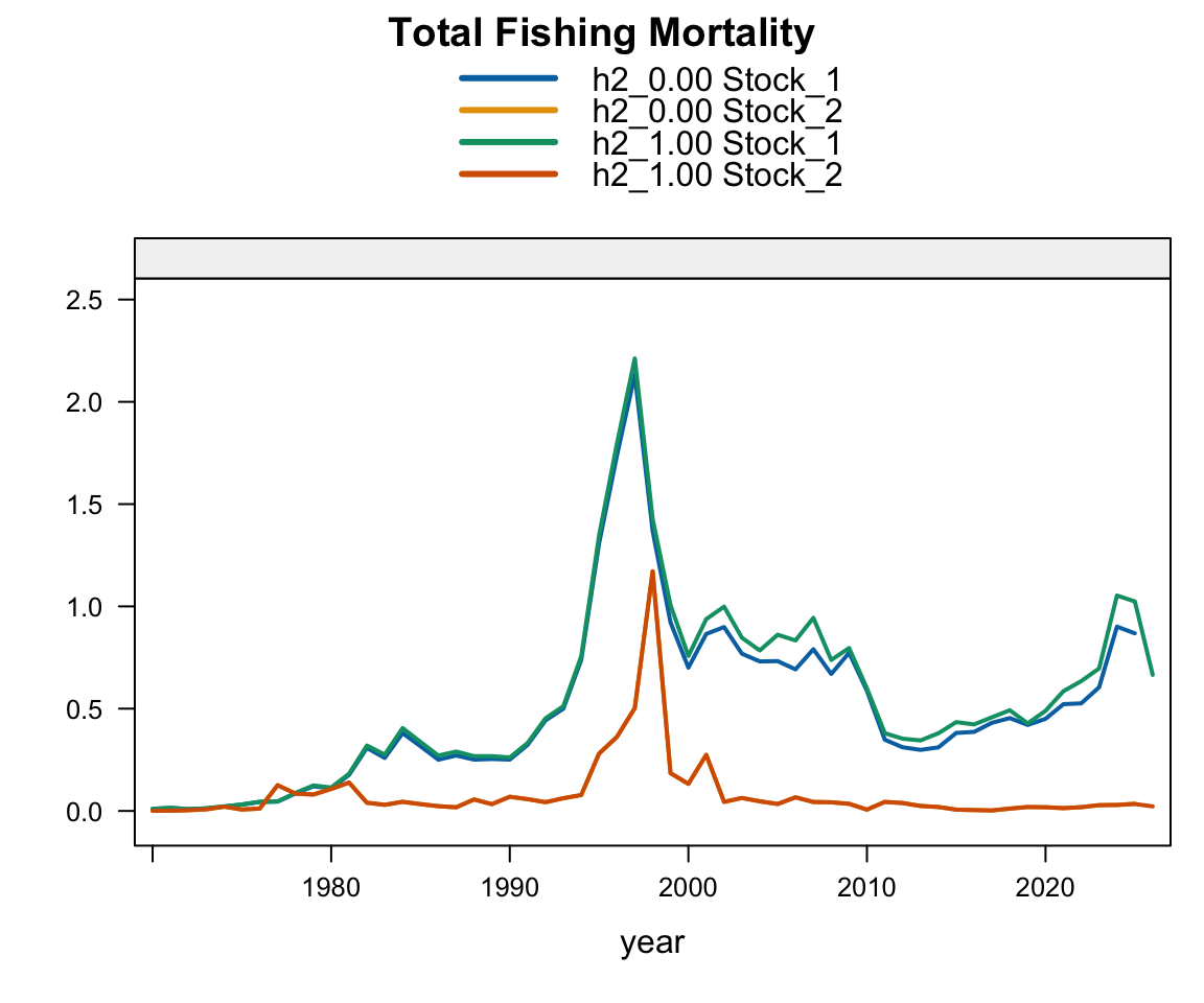
Plot comparing fishing mortality estimated by last year’s model (h2_0.00) to this year’s (h2_1.00).

Plot comparing fishing mortality estimated by last year’s model (h2_0.00) to this year’s (h2_1.00).

7 Sensitivity Analyses

7.1 Impact of only 2026 catch projections

How much of stock biomass trend is driven by incomplete fishery data? Only updates catch projections to 2026, using 2025 selectivity patterns and weights at age.
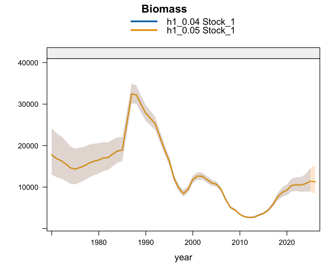
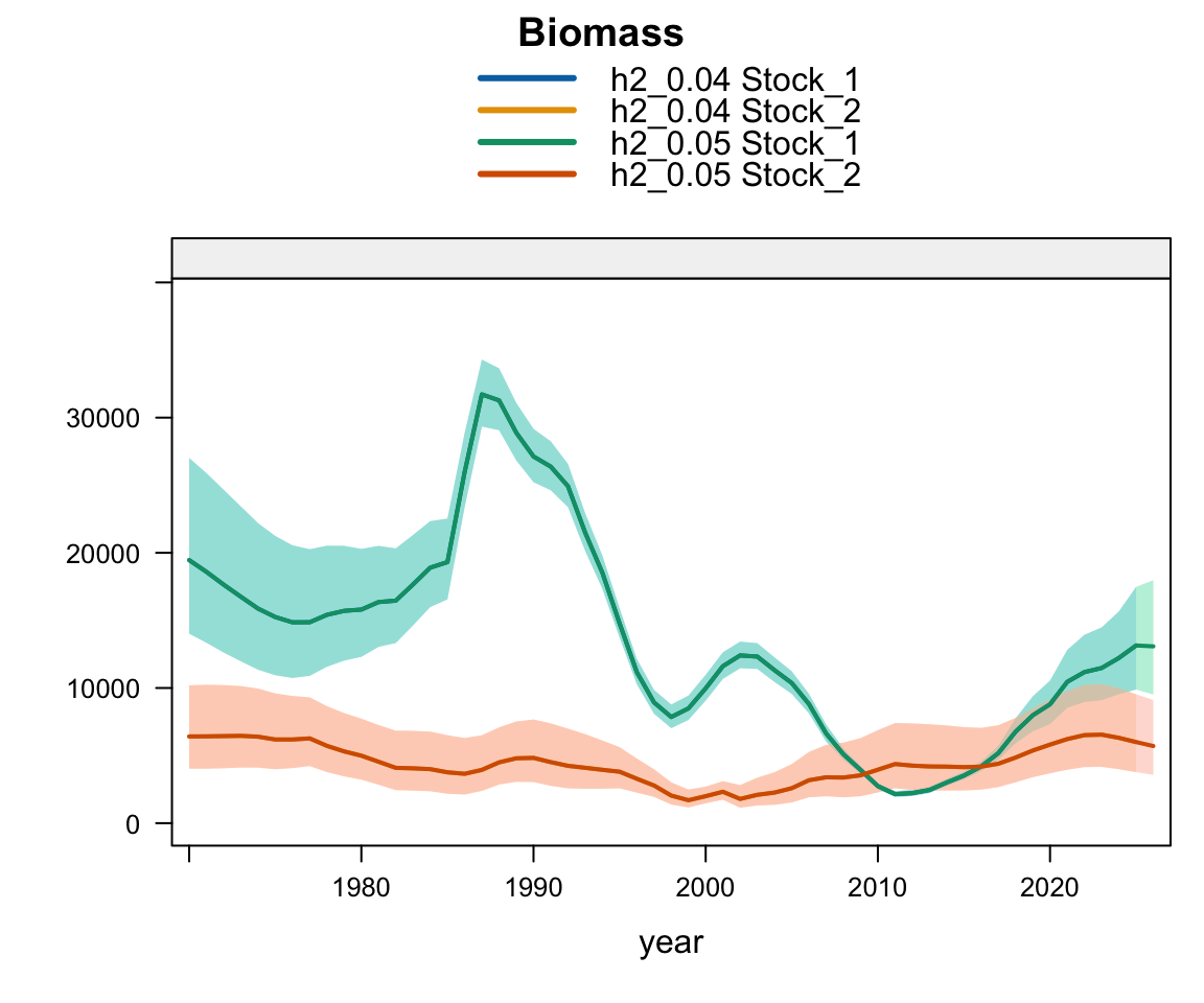
Plot comparing biomass estimates from using only 2026 catch projections.

Plot comparing biomass estimates from using only 2026 catch projections.

Plot comparing biomass estimates from using only 2026 catch projections.

Plot comparing biomass estimates from using only 2026 catch projections.

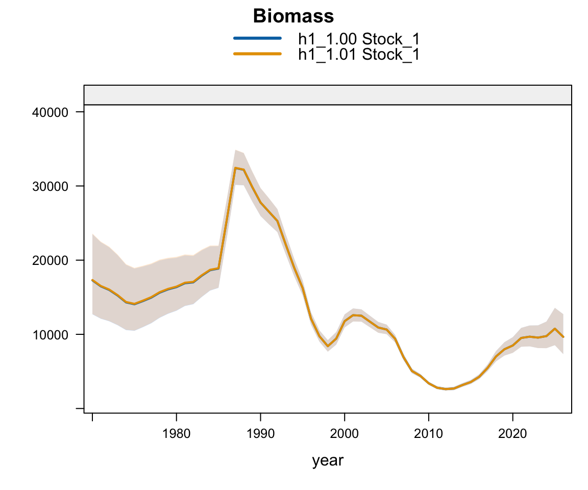
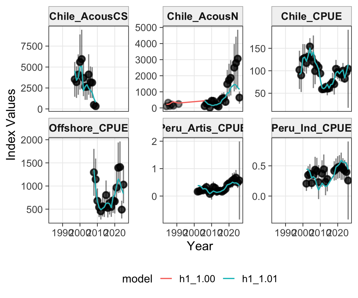
7.2 Removing early years of Chile_AcousN survey data

These years were very long ago (pre-2000) and the data still have an impact on the assessment. We don’t like them and want them to go away.
7.2.1 Single-stock hypothesis

Plot comparing biomass estimates from removing the early years of Chile’s acoustic survey data.

Plot comparing biomass estimates from removing the early years of Chile’s acoustic survey data.

7.2.2 Two-stock hypothesis

Plot comparing biomass estimates from removing the early years of Chile’s acoustic survey data.

Plot comparing biomass estimates from removing the early years of Chile’s acoustic survey data.

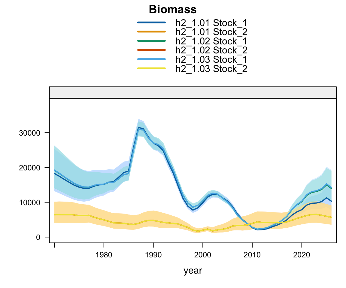
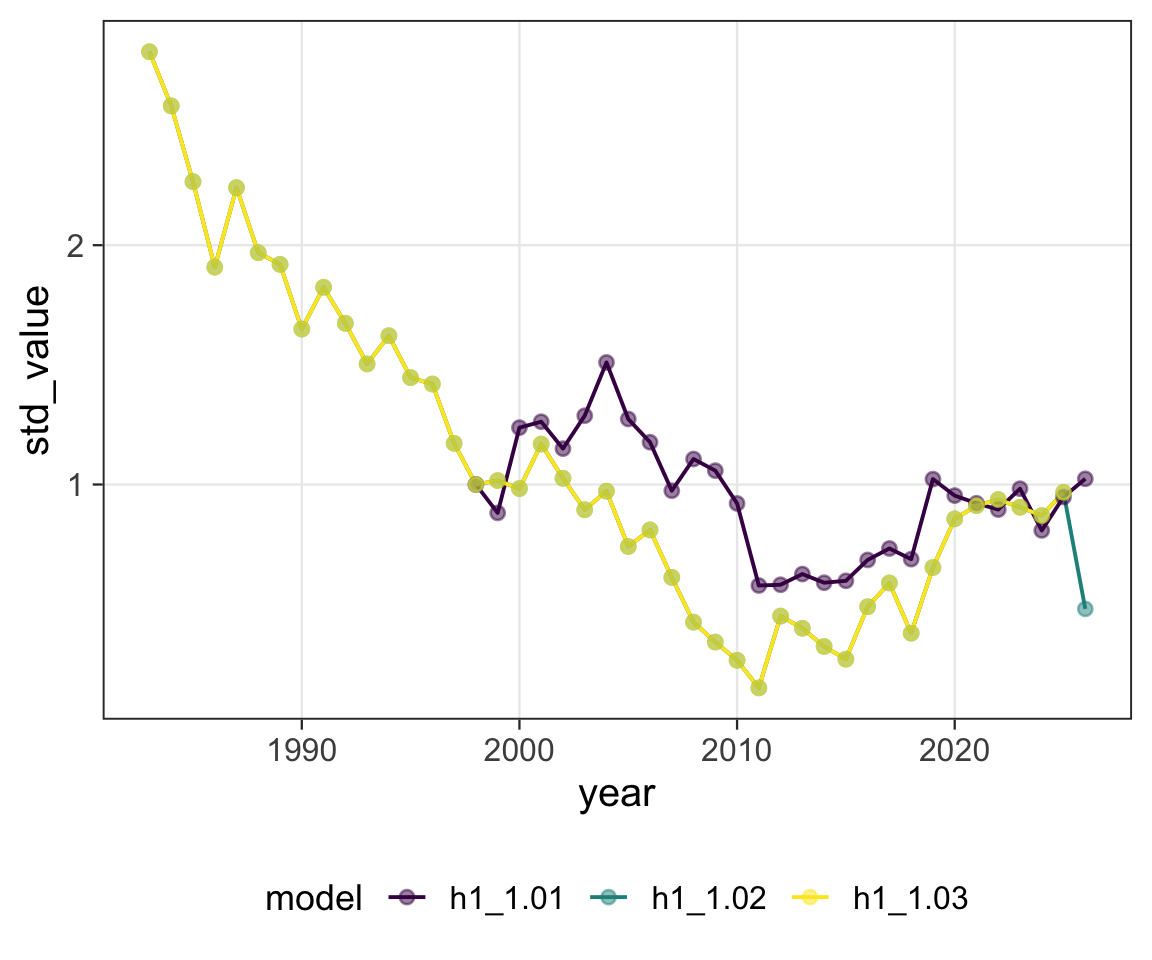
7.3 Traditional Chile CPUE

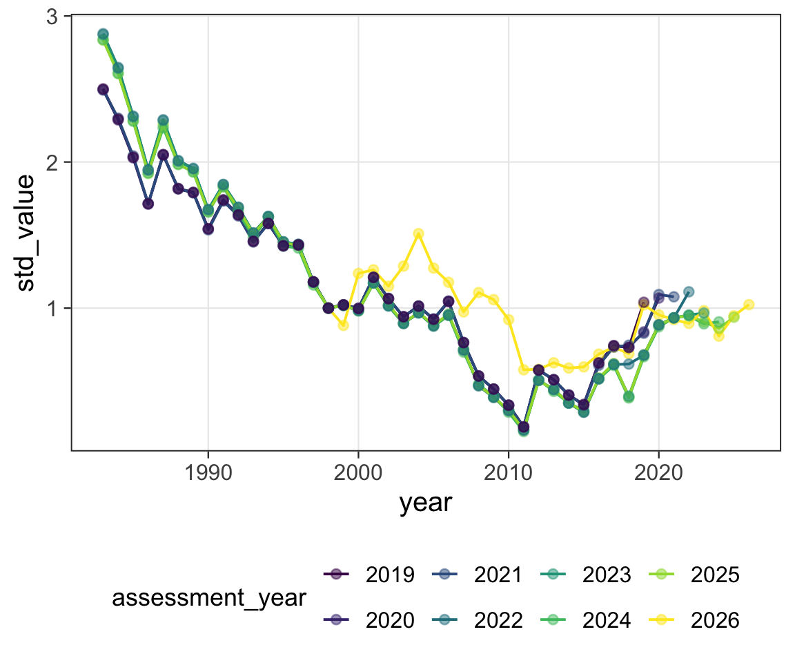
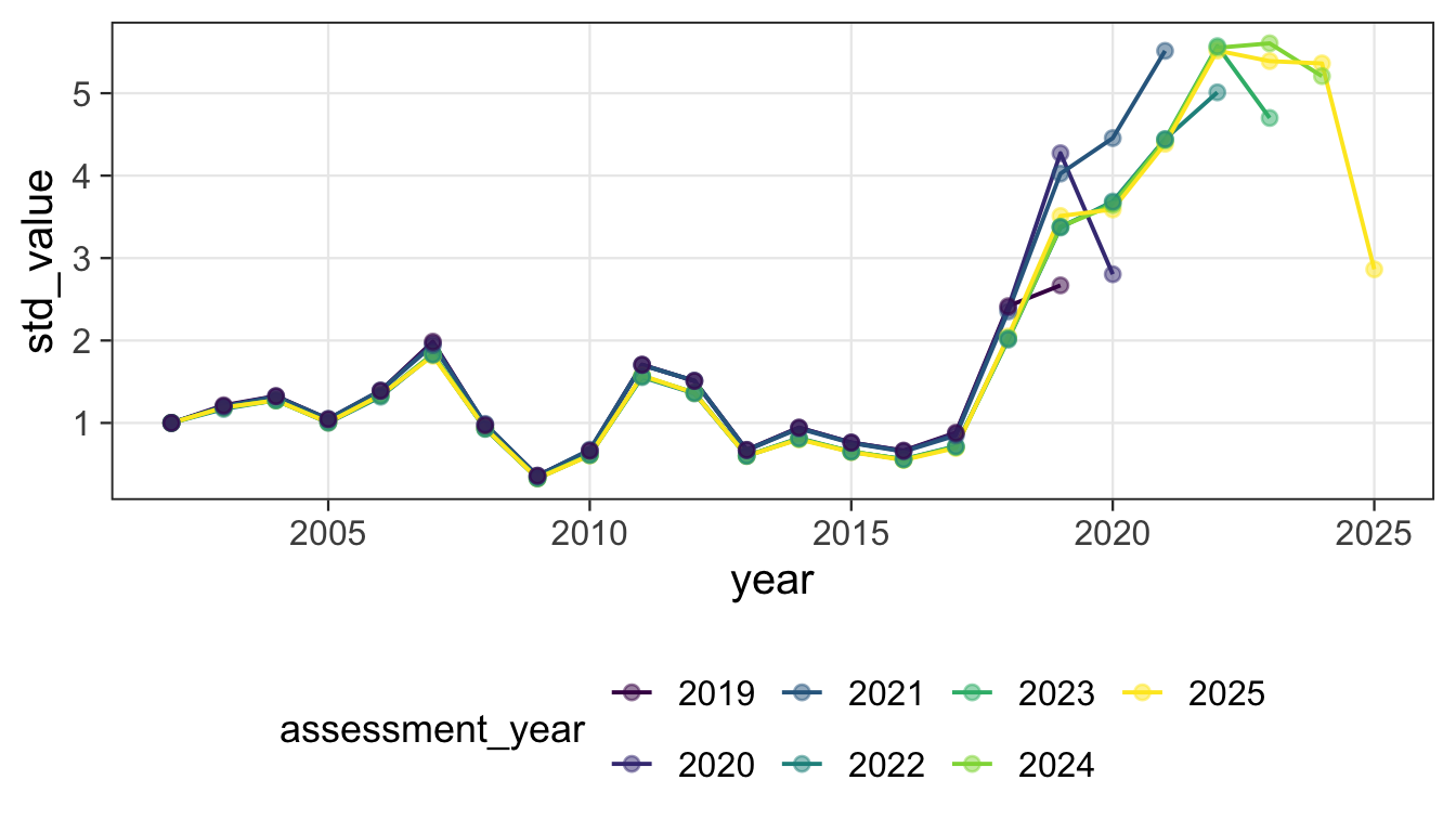
The Chile CPUE index was replaced during the 2026 benchmark SCW16. The new CPUE series has a strange trend in the most recent years, and we were interested to have a comparison with the old CPUE series calculated based on fishing trips (SC14-JM15).
7.3.0.1 Single-stock

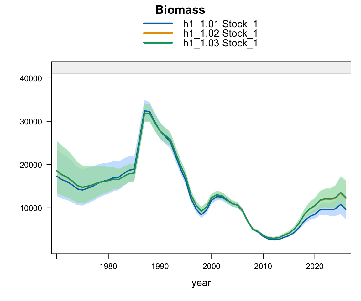
Plot comparing biomass estimates from using the CPUE based on fishing trips, with and without the present year’s data point (1.02 and 1.03 respectively).

Plot comparing biomass estimates from using the CPUE based on fishing trips, with and without the present year’s data point (1.02 and 1.03 respectively).

7.3.0.2 Two-stock hypothesis

Plot comparing biomass estimates from using the CPUE based on fishing trips, with and without the present year’s data point (1.02 and 1.03 respectively).

Plot comparing biomass estimates from using the CPUE based on fishing trips, with and without the present year’s data point (1.02 and 1.03 respectively).

7.4 Offshore Weight at Age

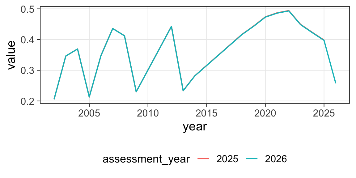
The weights at age for the offshore fleet in 2025 and 2026 were unusually low. A mean of the previous five years (2019-2024) were used to replace those values, until the data can be re-examined and corrected.

7.4.1 Biomass

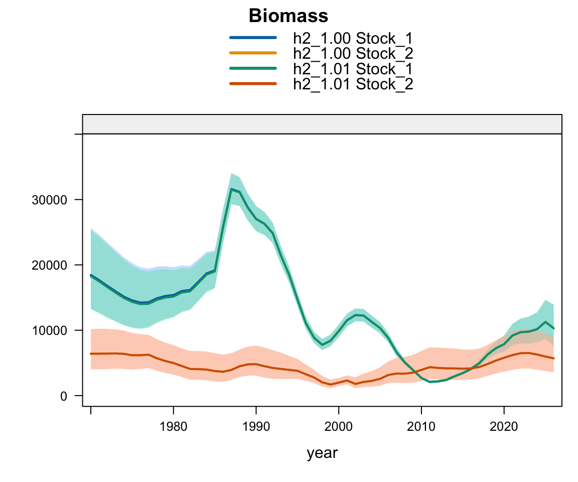
Plot comparing biomass estimates from using the average weight at age across 2019-2024 for the offshore fleet in 2025 and 2026.

Plot comparing biomass estimates from using the average weight at age across 2019-2024 for the offshore fleet in 2025 and 2026.

Plot comparing biomass estimates from using the average weight at age across 2019-2024 for the offshore fleet in 2025 and 2026.

Plot comparing biomass estimates from using the average weight at age across 2019-2024 for the offshore fleet in 2025 and 2026.

7.5 High seas catch

In 2025, Chile caught 22,799 tons of jack mackerel in the SPRFMO Convention Area. Given the difference in selectivity patterns between the Chilean and the Offshore fleets, the proposal is to add that catch data to the Northern Chile fleet (model 1.05).

A similar occurrence happened in 2026, with Peru catching 10,000 tons of jack mackerel in the Convention Area.
7.5.1 Data

7.5.2 Biomass

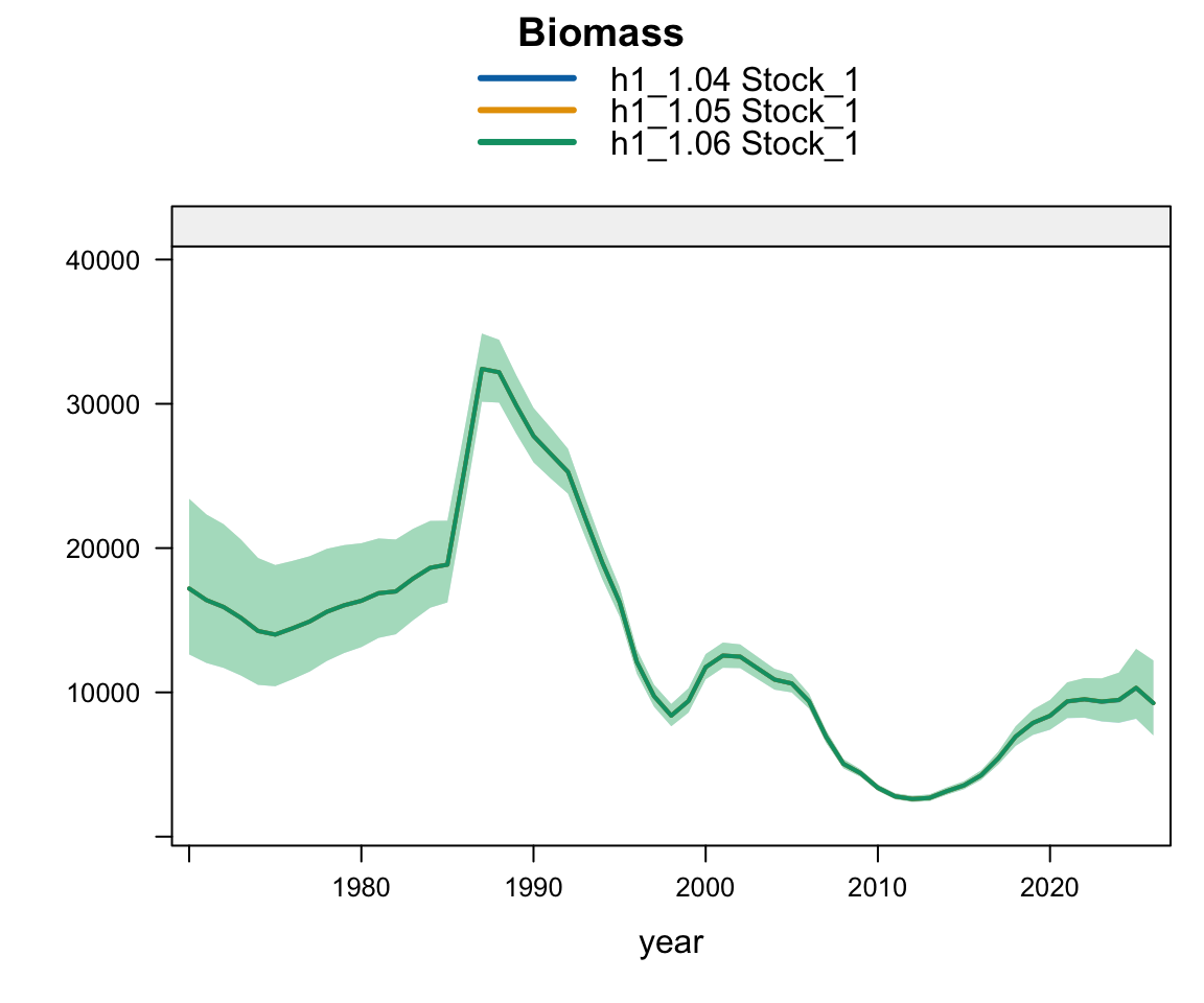
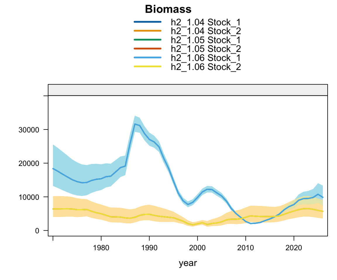
Plot comparing biomass estimates from adding 2025 high seas catch to the Northern Chile fleet (1.05) and 2026 high seas catch to the FarNorth fleet (1.06).

Plot comparing biomass estimates from adding 2025 high seas catch to the Northern Chile fleet (1.05) and 2026 high seas catch to the FarNorth fleet (1.06).

Plot comparing biomass estimates from adding 2025 high seas catch to the Northern Chile fleet (1.05) and 2026 high seas catch to the FarNorth fleet (1.06).

Plot comparing biomass estimates from adding 2025 high seas catch to the Northern Chile fleet (1.05) and 2026 high seas catch to the FarNorth fleet (1.06).

8 Final Model (PRELIMINARY)

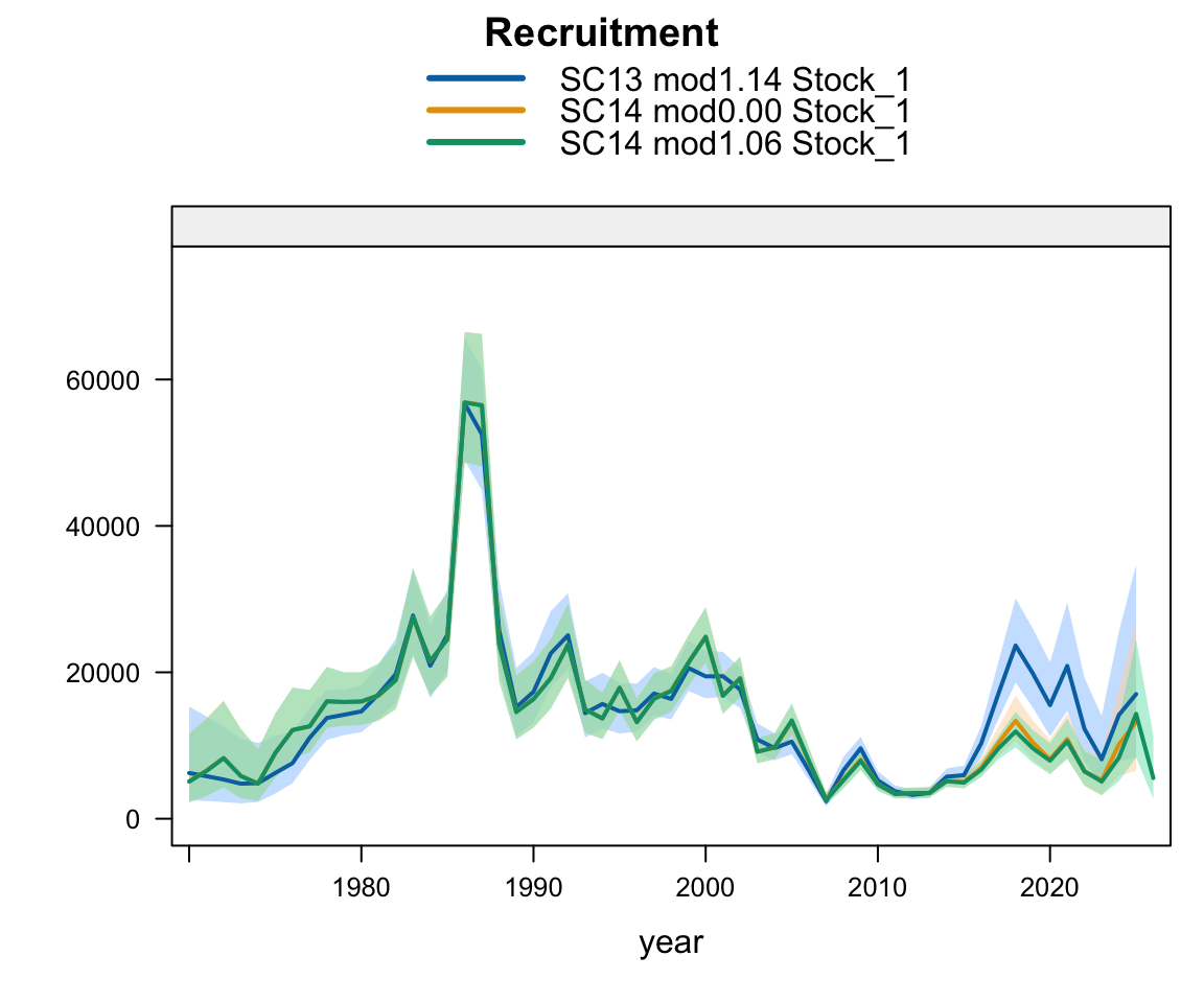
Model 1.06 was selected as the final model for 2026. This model incorporates data updated to 2025, flexibility in selectivity patterns for the SC Chile and Offshore fleets in 2025, and increased confidence (decreased CV) for the 2025 age composition data from the same fleets. The early years of Chile acoustic north survey data were downweighted, and the changes in Peruvian weight at age for older fish were corrected.
8.1 Comparison to last year

8.1.1 Single-stock hypothesis

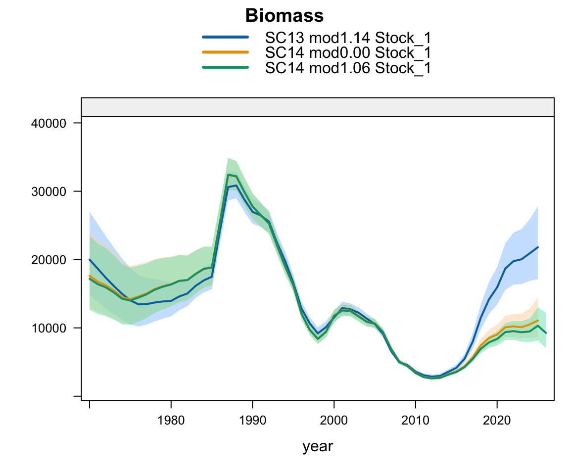
Plot comparing biomass estimates from last year’s model with the final model selected for this year.

Plot comparing biomass estimates from last year’s model with the final model selected for this year.

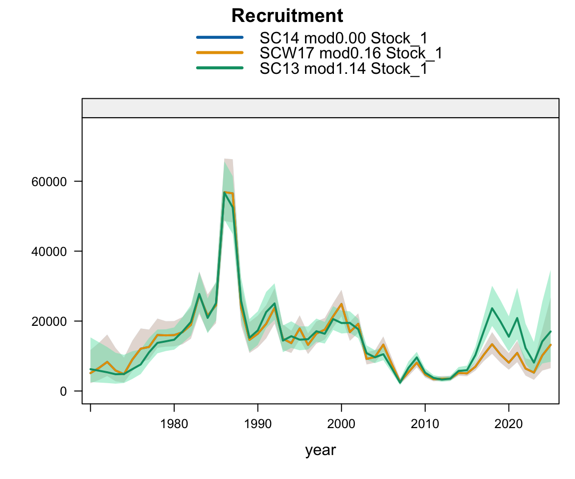
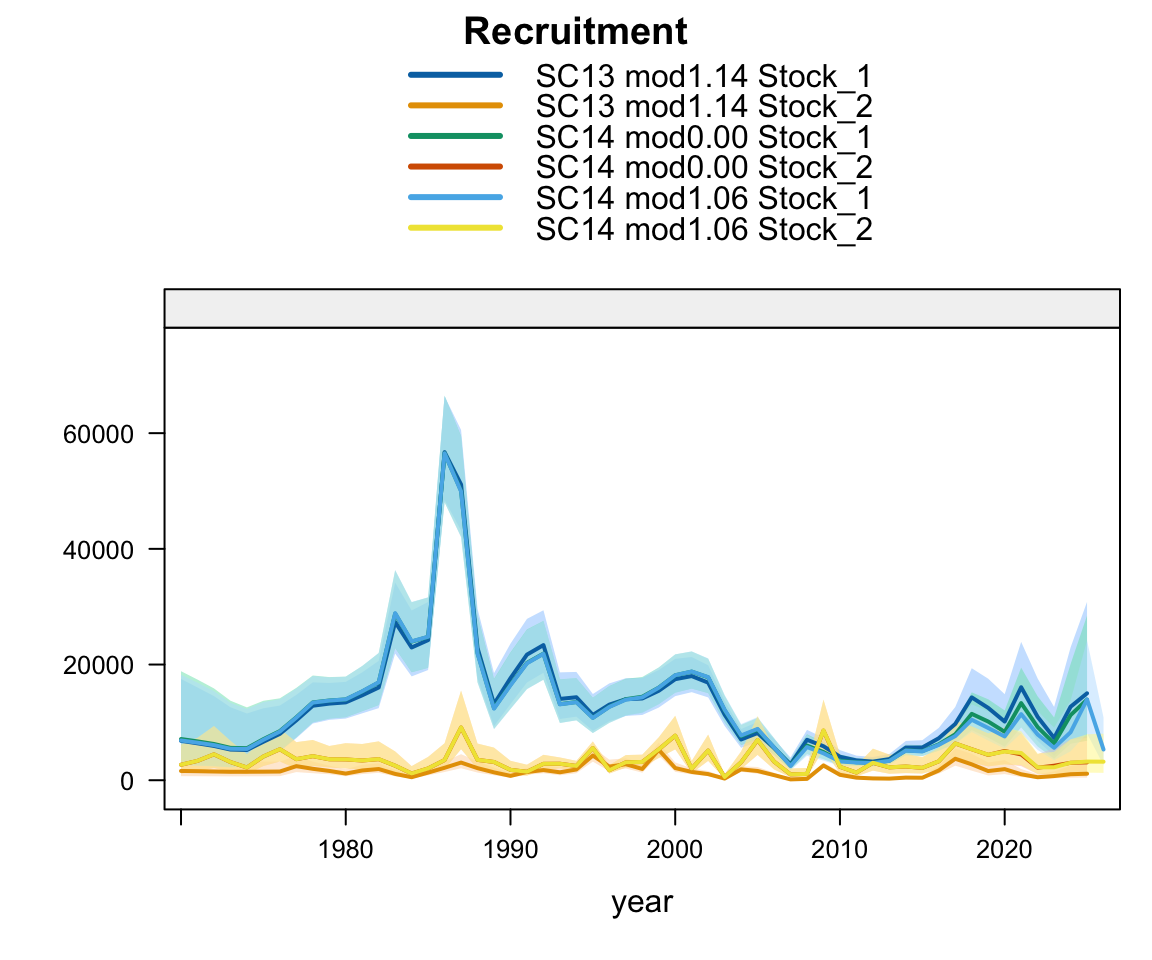
Plot comparing recruitment estimates from last year’s model with the final model selected for this year.

Plot comparing recruitment estimates from last year’s model with the final model selected for this year.

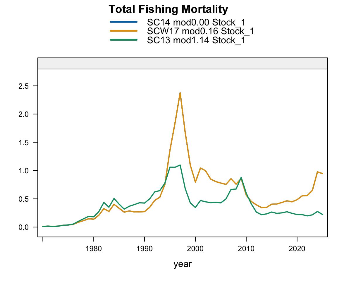
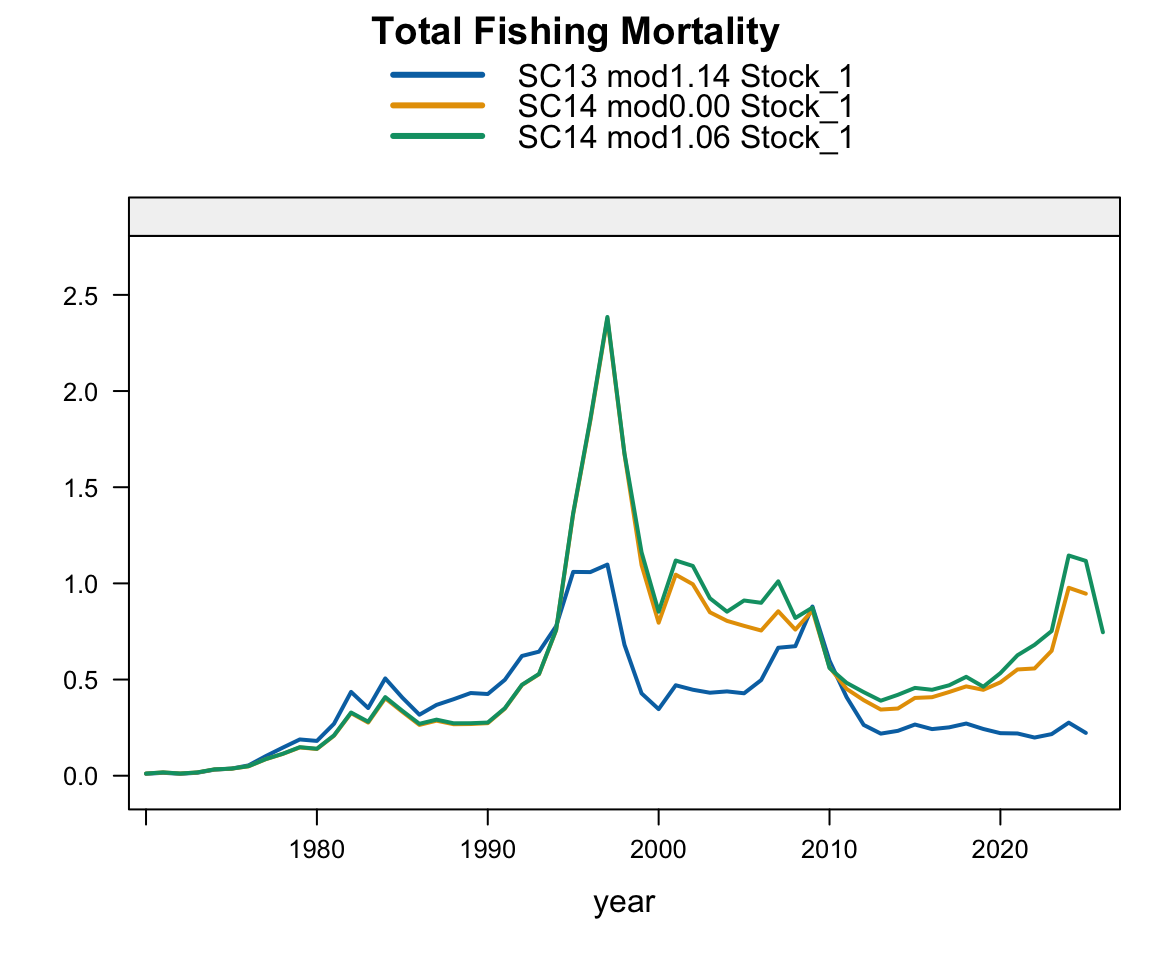
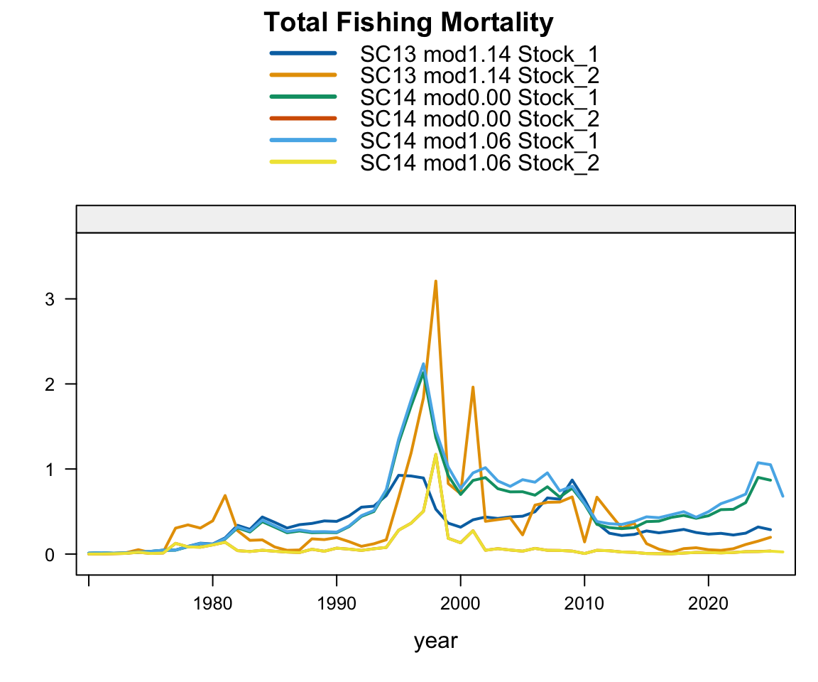
Plot comparing fishing mortality estimates from last year’s model with the final model selected for this year.

Plot comparing fishing mortality estimates from last year’s model with the final model selected for this year.

8.1.2 Two-stock hypothesis

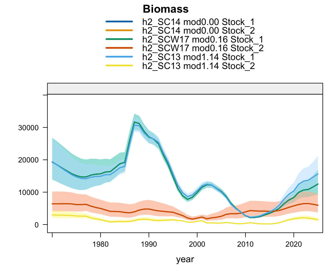
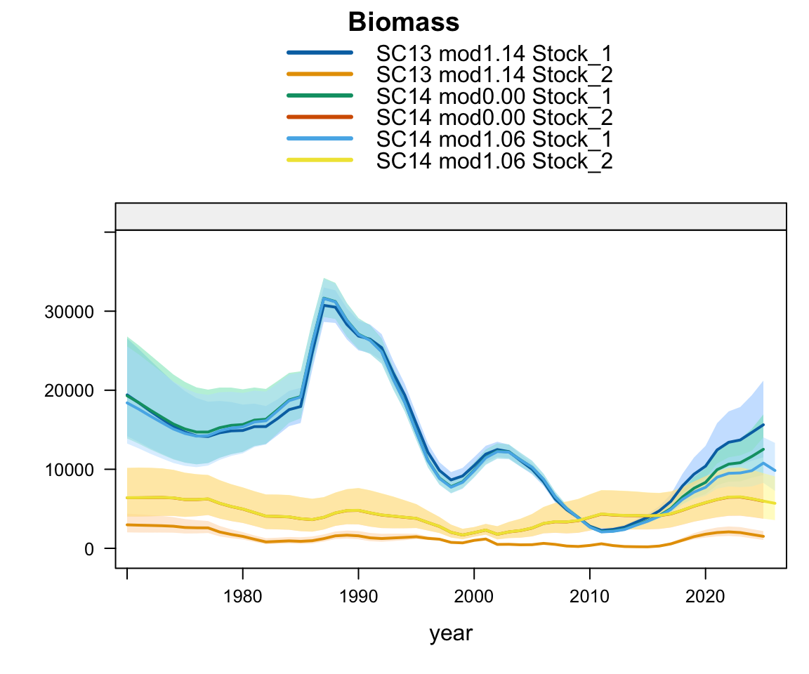
Plot comparing biomass estimates from last year’s model with the final model selected for this year.

Plot comparing biomass estimates from last year’s model with the final model selected for this year.

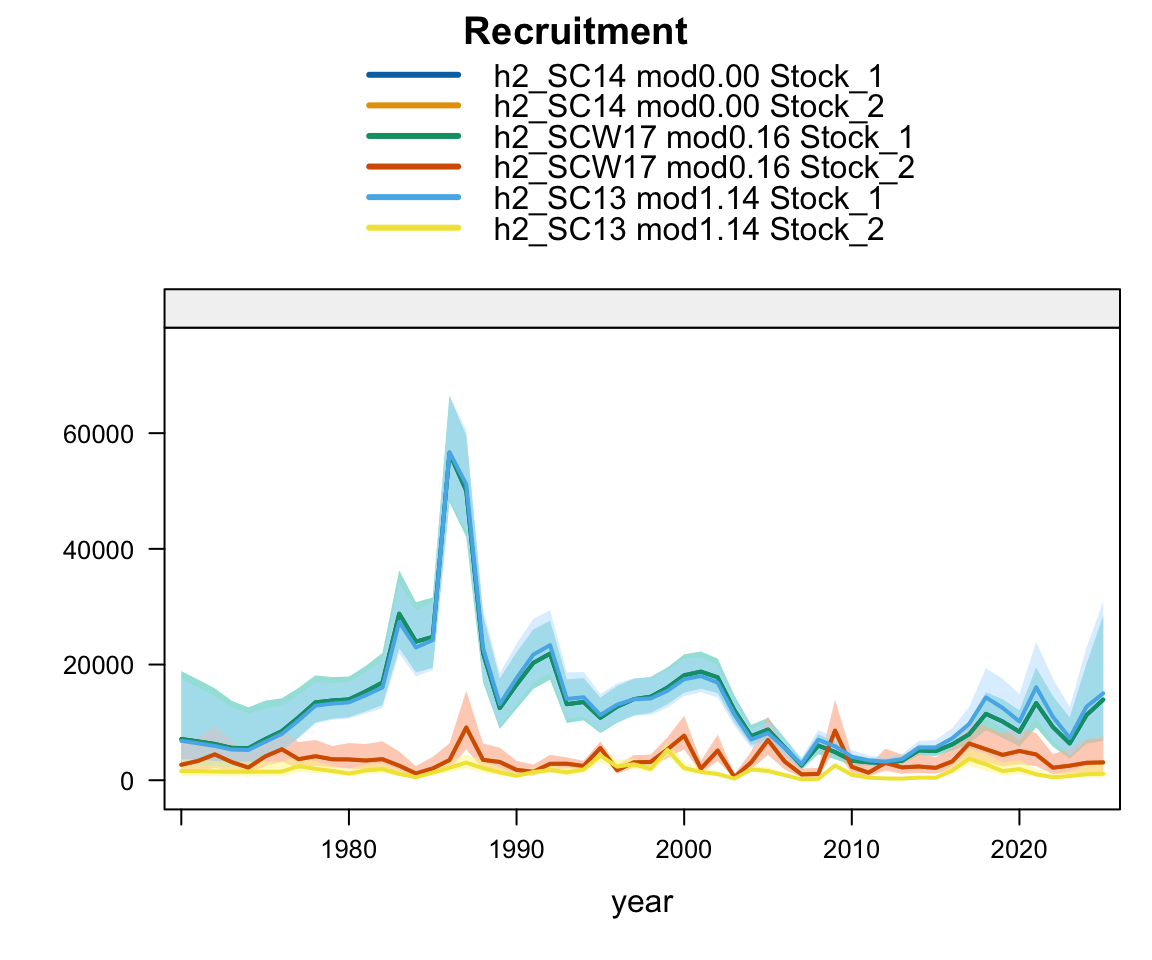
Plot comparing recruitment estimates from last year’s model with the final model selected for this year.

Plot comparing recruitment estimates from last year’s model with the final model selected for this year.

Plot comparing fishing mortality estimates from last year’s model with the final model selected for this year.

Plot comparing fishing mortality estimates from last year’s model with the final model selected for this year.

8.2 Model Diagnostics

8.2.1 Single-Stock Hypothesis

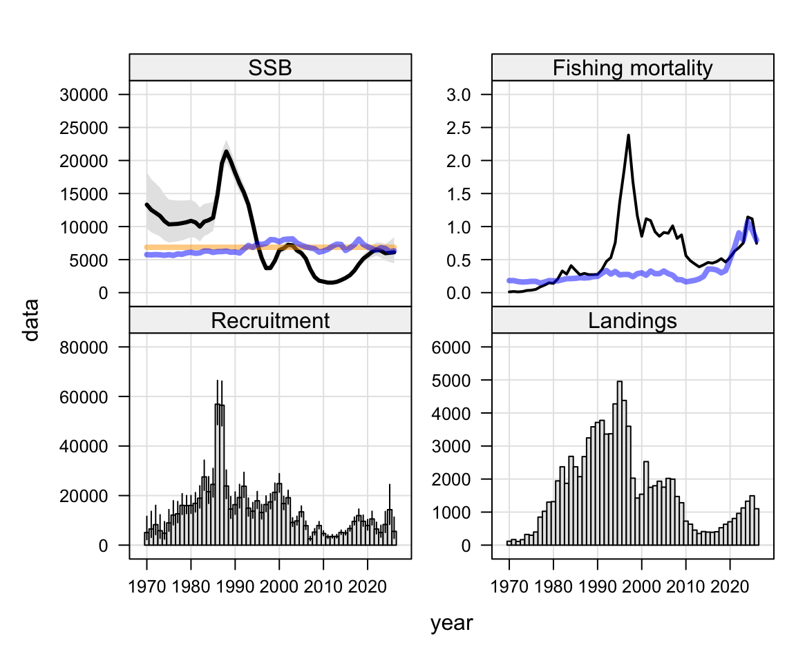
The \(B_{MSY}\) for this year (an average of the most recent ten years) will be 6.869 million tons.
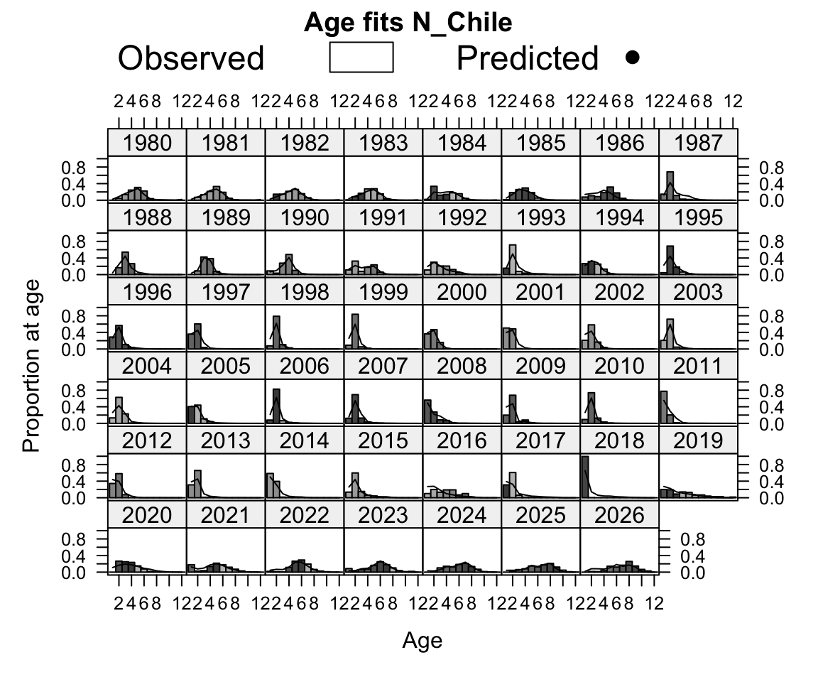
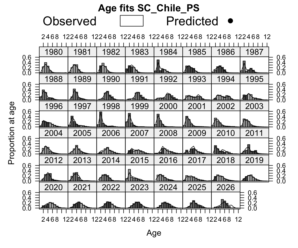
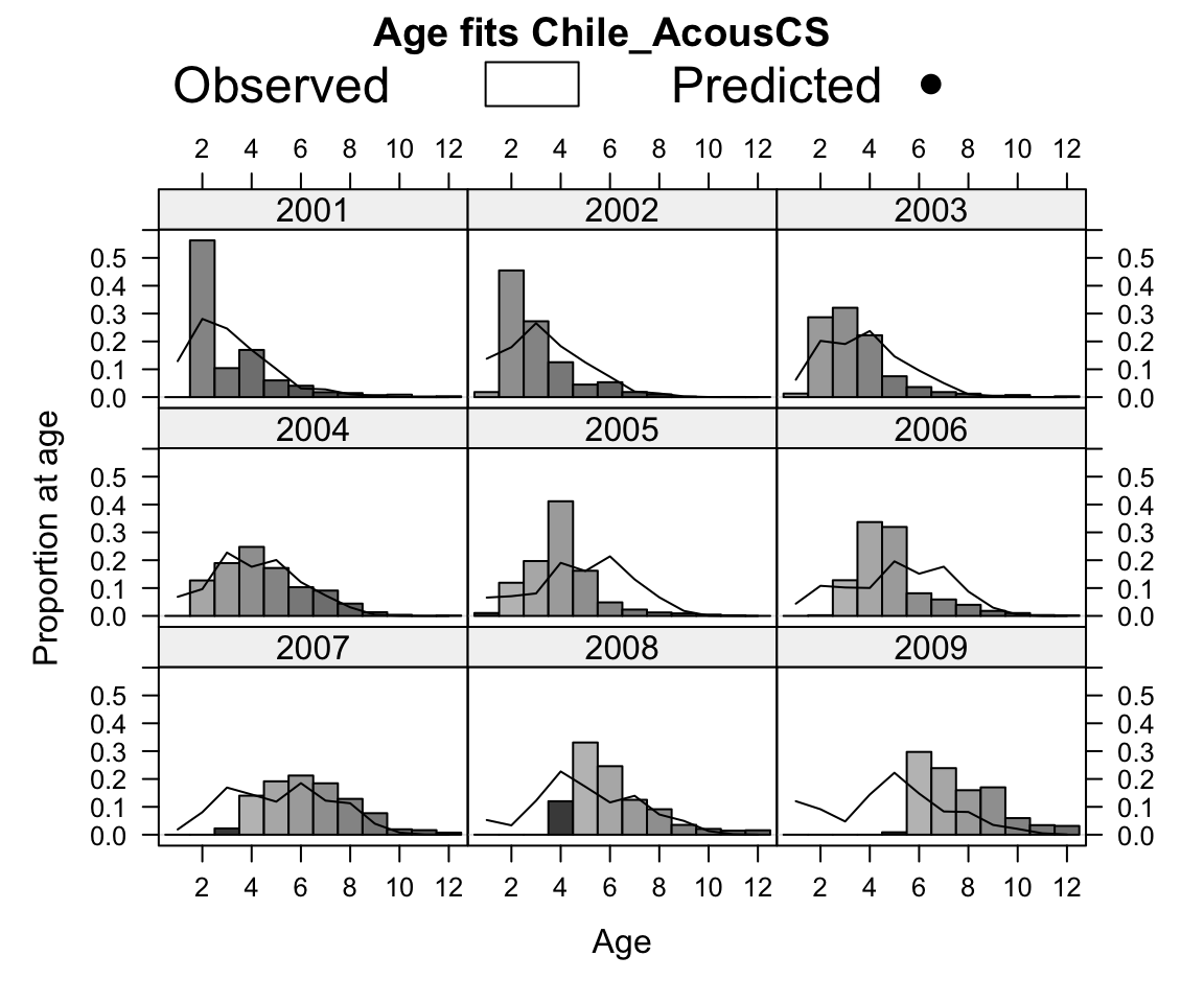
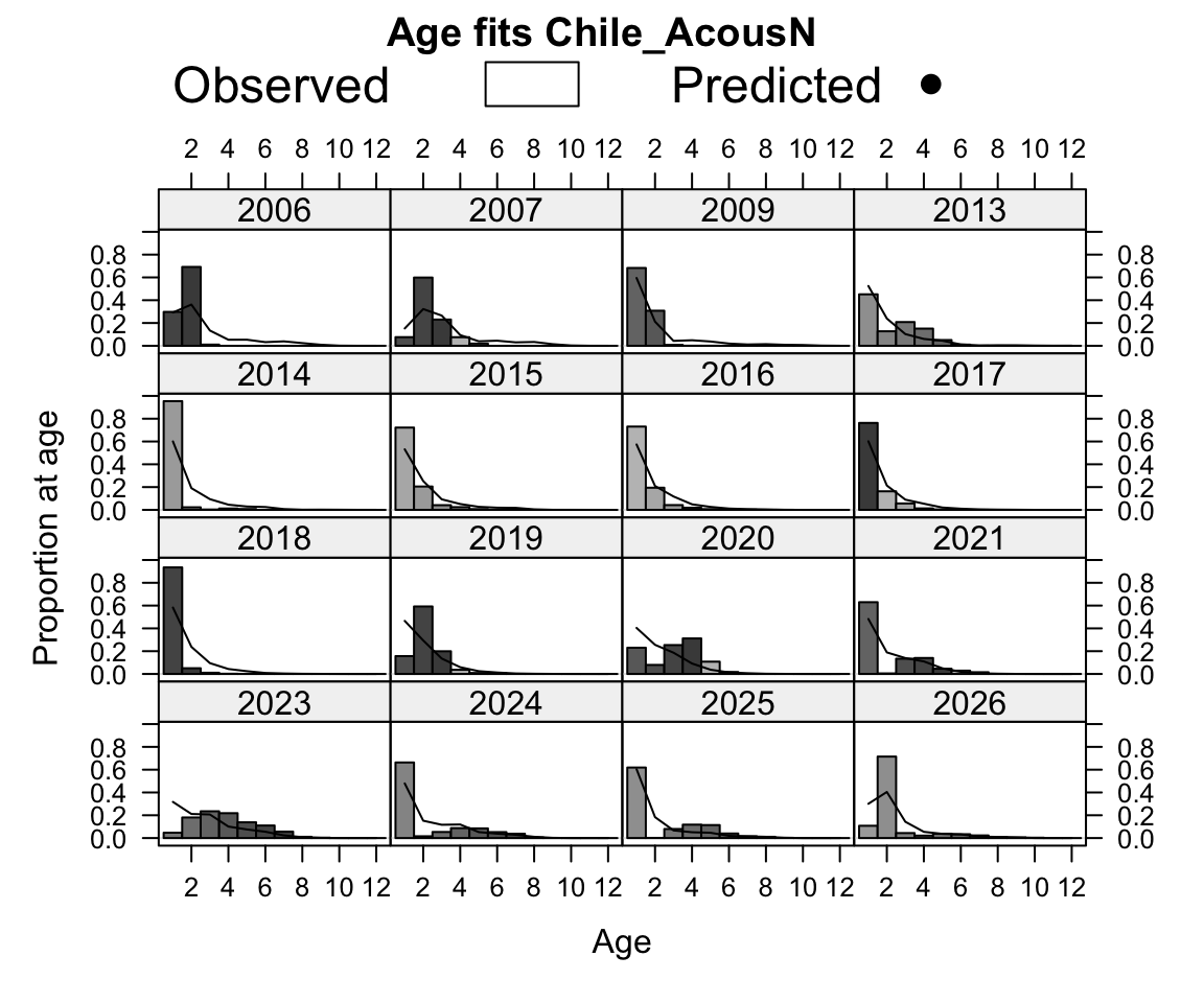
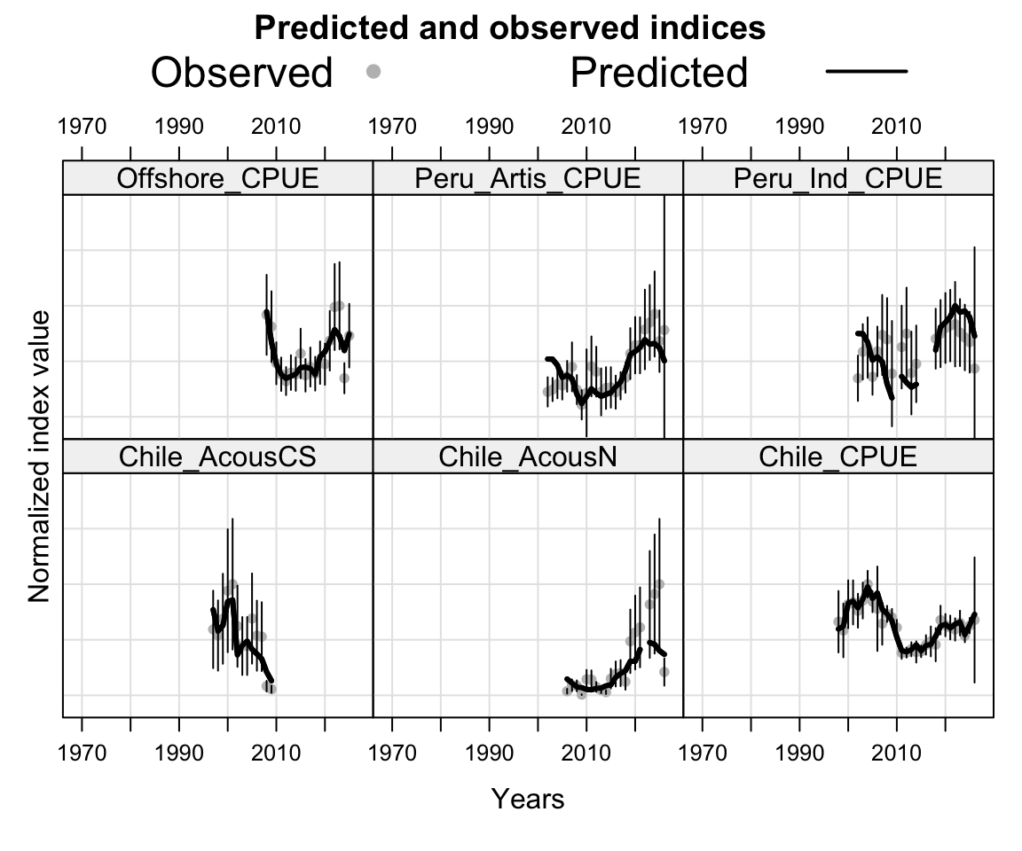
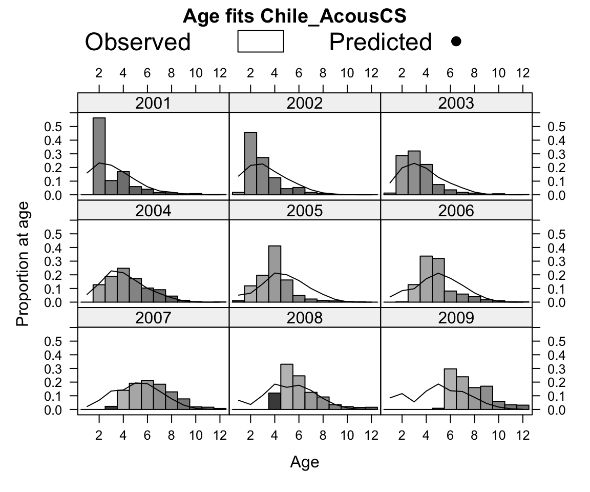
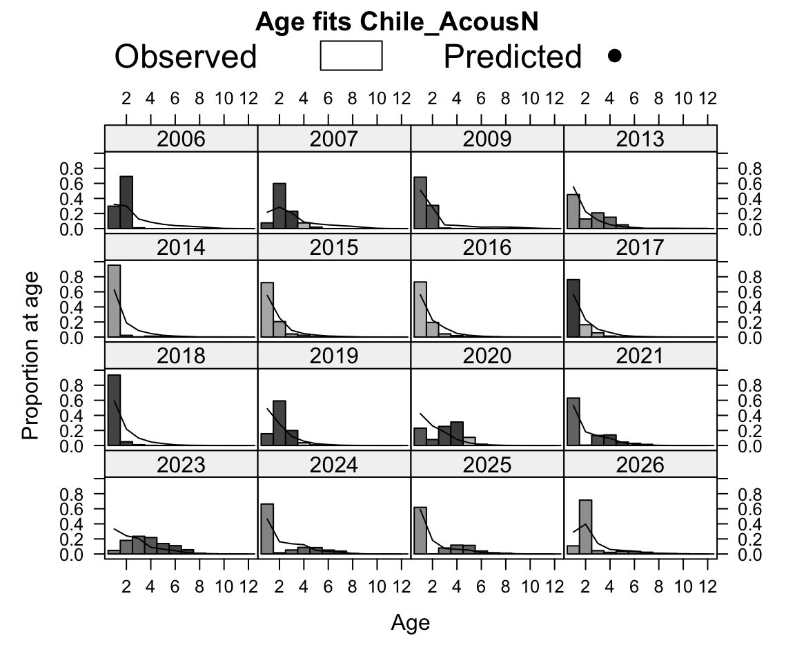
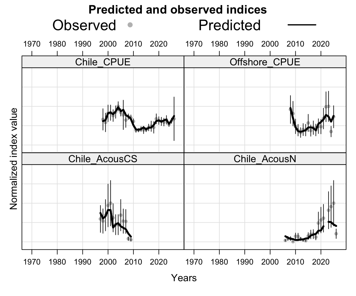
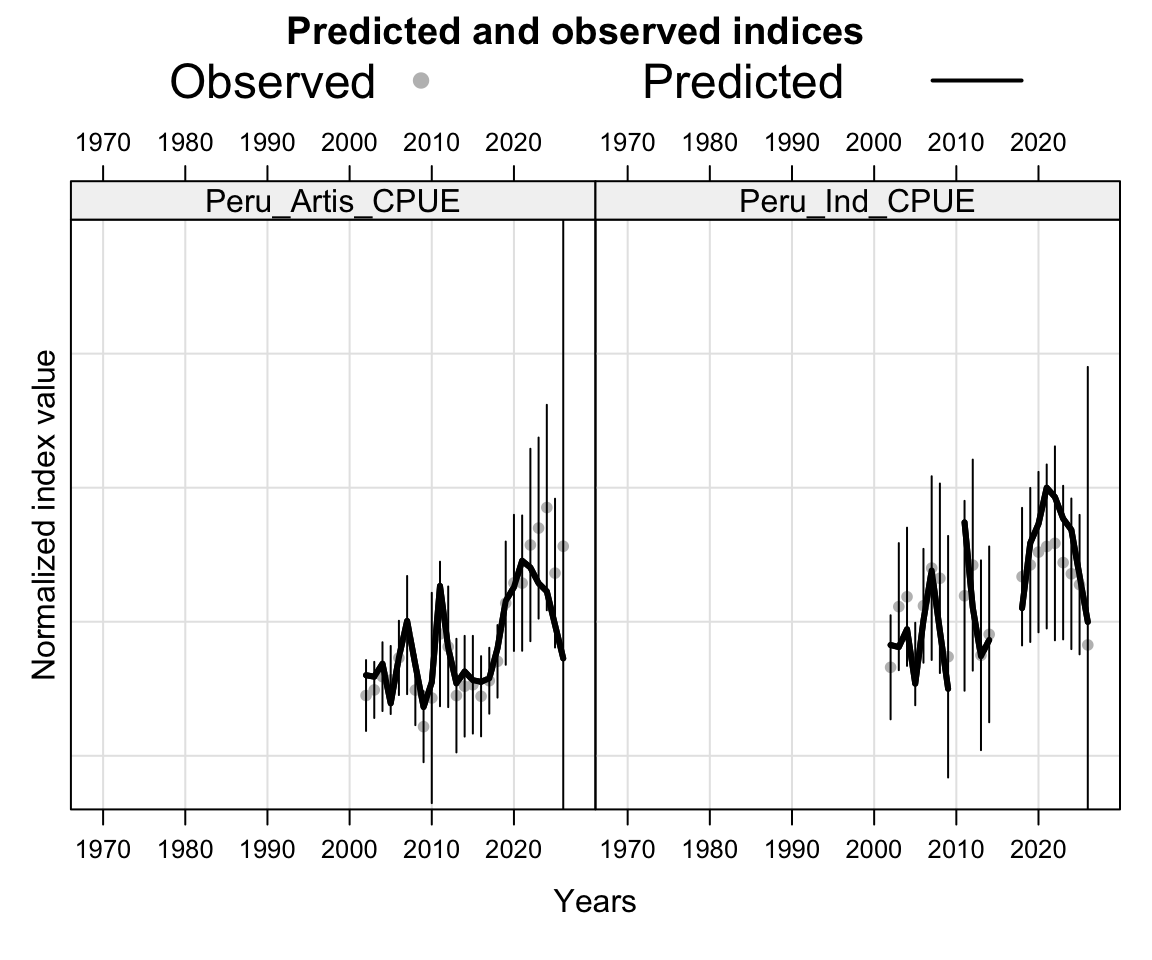
8.2.1.1 Fits to Data

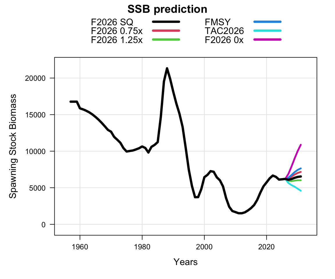
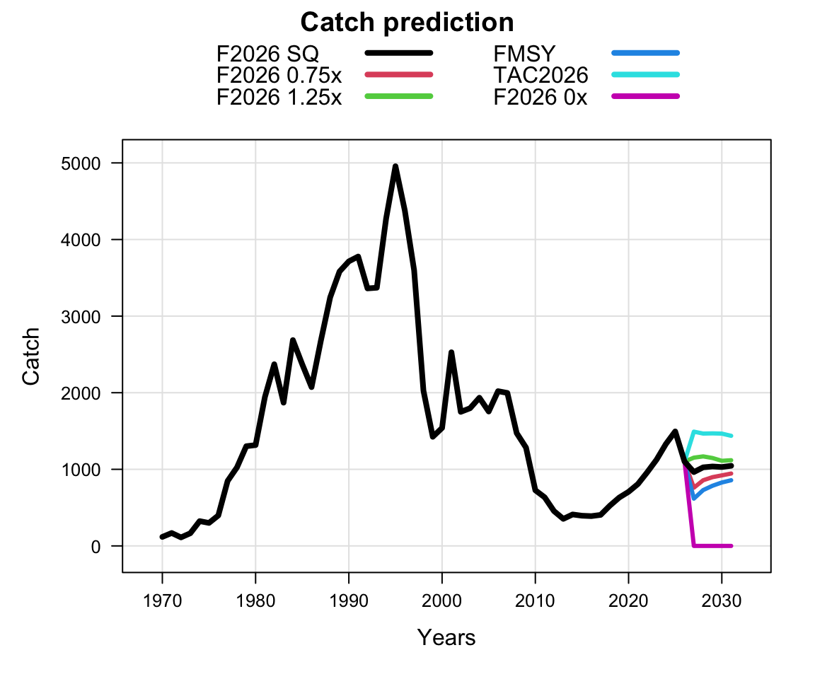
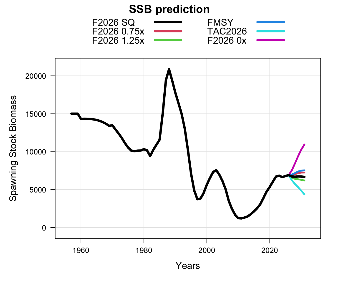
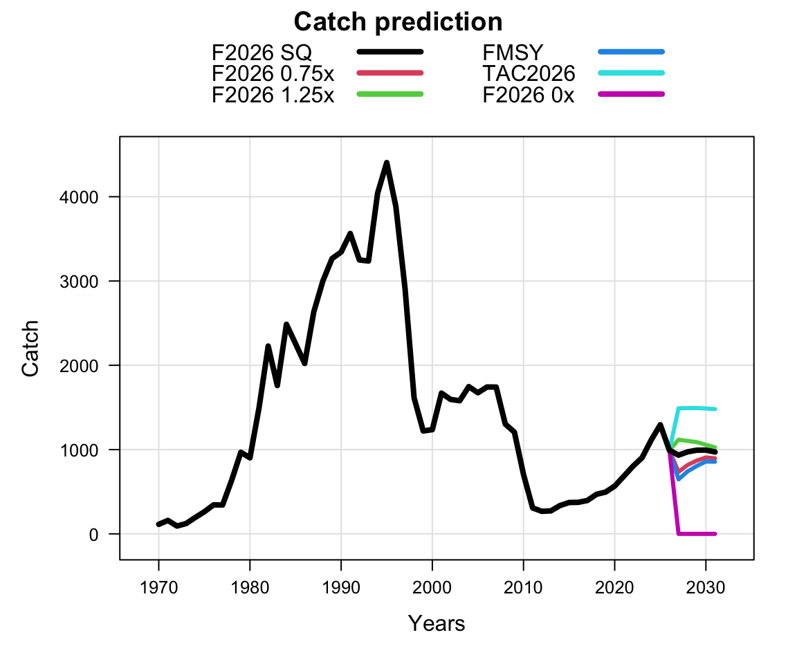
8.2.1.2 Projections

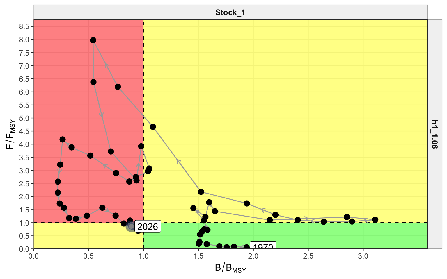
8.2.1.3 Kobe Plot

BMSY fixed at 6.869 million tons.

BMSY fixed at 6.869 million tons.

8.2.1.4 Kobe Plot (with dynamic BMSY)

The dynamic reference point uses each year’s model-estimated \(B_{MSY}/B_0\) ratio multiplied by that year’s unfished spawning biomass. Fishing mortality remains relative to the model-estimated \(F_{MSY}\). The first model year is omitted because the saved unfished-biomass ratio begins in the following year.
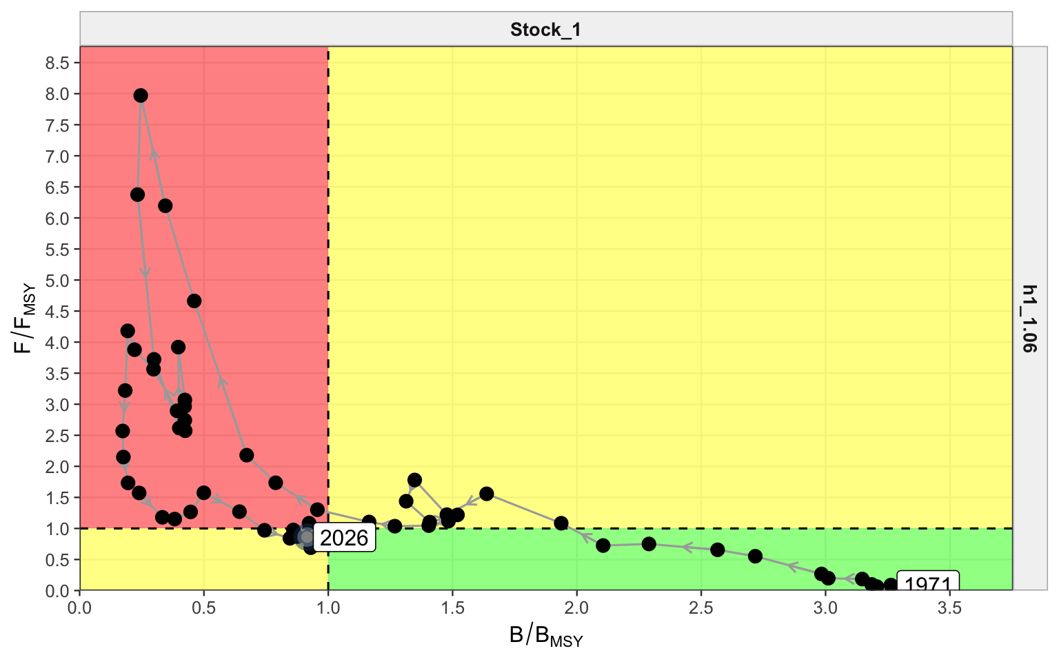
Annual stock-status trajectory with spawning biomass relative to dynamic BMSY on the horizontal axis and fishing mortality relative to FMSY on the vertical axis.

Kobe trajectory relative to annual dynamic BMSY and model-estimated FMSY.

8.2.1.5 Summary Plot

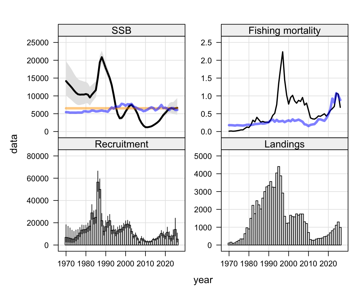
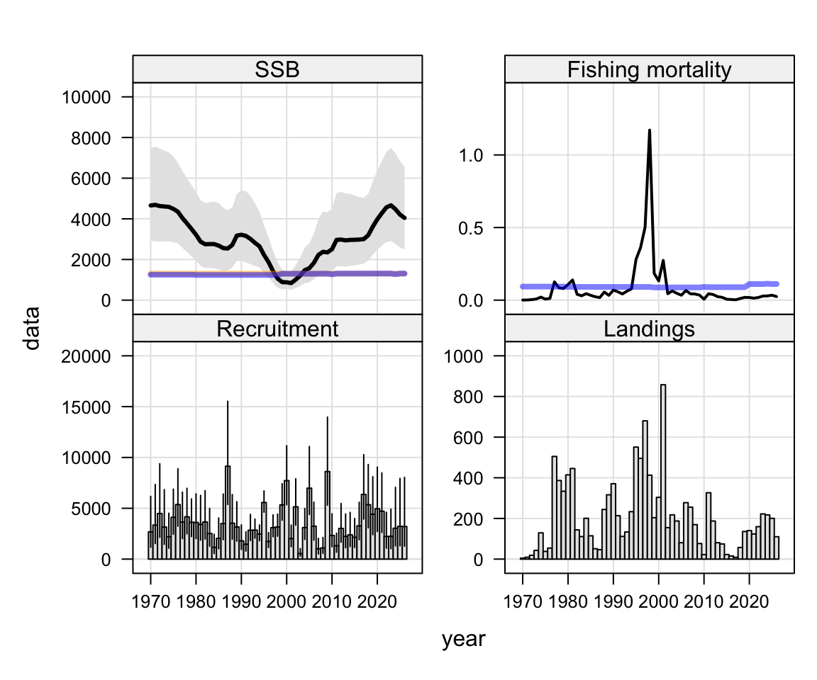
BMSY is fixed at 6.869 million tons, shown by the orange line. The blue lines show the MSY values (BMSY and FMSY) estimated annually within the model.

BMSY is fixed at 6.869 million tons, shown by the orange line. The blue lines show the MSY values (BMSY and FMSY) estimated annually within the model.

8.2.2 Two-Stock Hypothesis

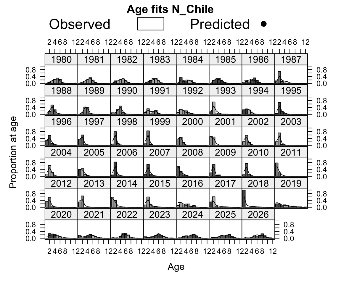
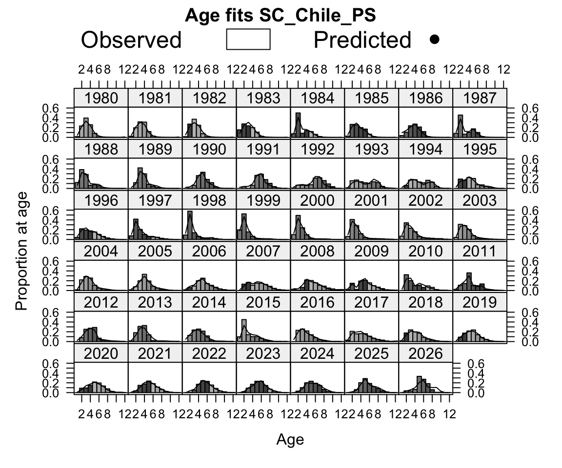
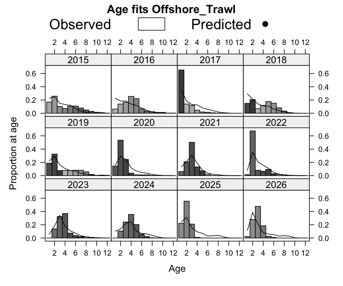
The \(B_{MSY}\) for this year (an average of the most recent ten years) will be 6.524 million tons for the south stock and 1.305 million tons for the north stock.
8.2.2.1 Fits to Data

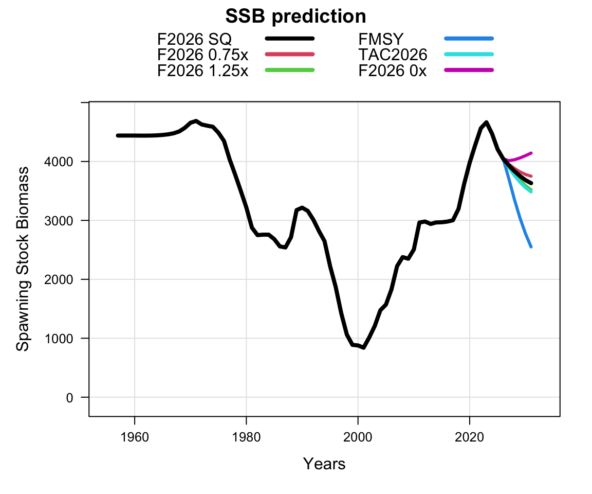
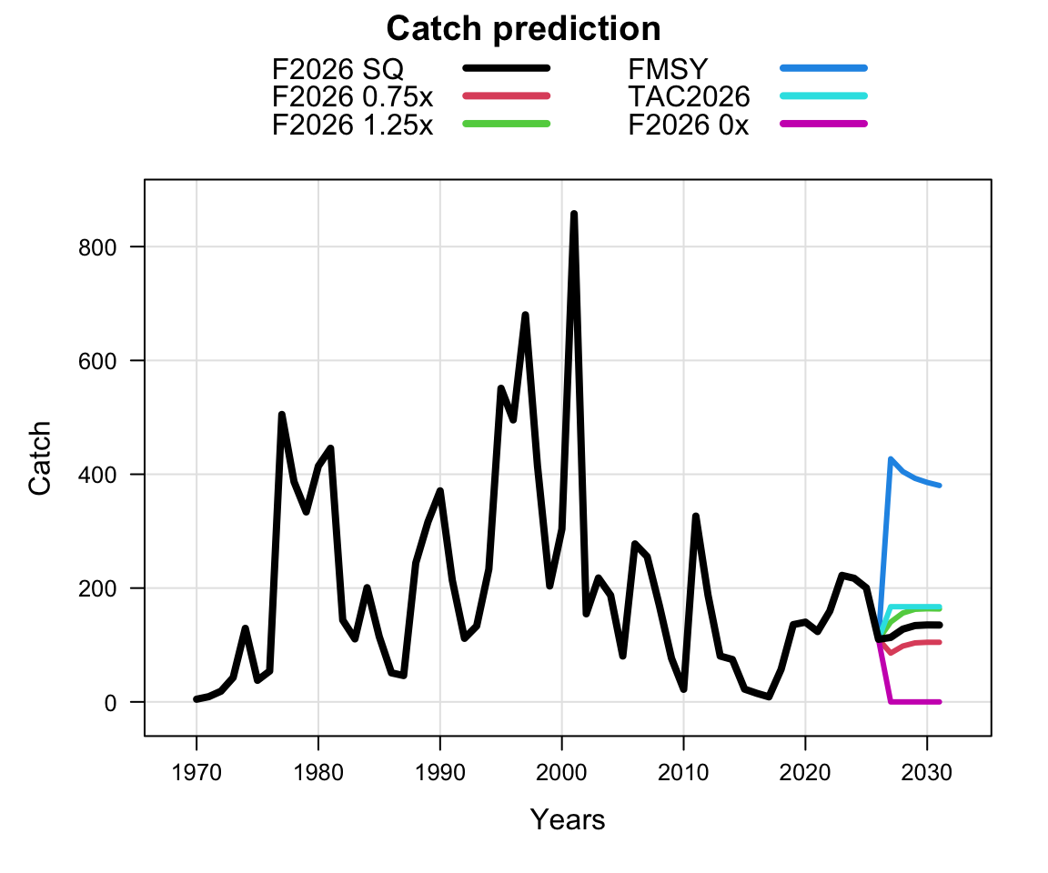
8.2.2.2 Projections

8.2.2.3 Kobe Plot

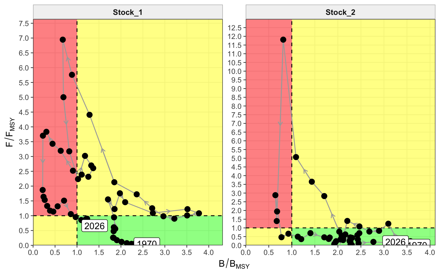
BMSY fixed at 6.524 million tons for the south stock and 1.305 million tons for the north stock.
BMSY fixed at 6.524 million tons for the south stock and 1.305 million tons for the north stock.
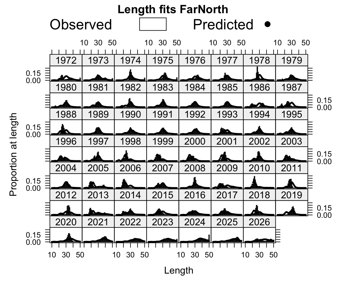
8.2.2.4 Summary Plot

BMSY fixed at 6.524 million tons for the south stock and 1.305million tons for the north stock, shown as the orange line. The blue lines show the MSY values (BMSY and FMSY) estimated annually within the model.

BMSY fixed at 6.524 million tons for the south stock and 1.305million tons for the north stock, shown as the orange line. The blue lines show the MSY values (BMSY and FMSY) estimated annually within the model.

BMSY fixed at 6.524 million tons for the south stock and 1.305million tons for the north stock, shown as the orange line. The blue lines show the MSY values (BMSY and FMSY) estimated annually within the model.

BMSY fixed at 6.524 million tons for the south stock and 1.305million tons for the north stock, shown as the orange line. The blue lines show the MSY values (BMSY and FMSY) estimated annually within the model.

8.3 Likelihood Table

h1_1.06 h2_1.06
catch_like 1.46 0.63
age_like_fsh 290.83 262.10
length_like_fsh 572.38 481.54
sel_like_fsh 268.08 251.24
ind_like 163.02 137.70
age_like_ind 67.92 68.20
length_like_ind 0.00 0.00
sel_like_ind 16.86 16.50
rec_like 3.99 5.21
fpen 0.00 0.06
post_priors_indq 0.22 0.19
post_priors 0.00 0.00
residual 0.00 0.00
total 1384.75 1223.38

9 Other Business

9.1 Data needs

9.2 General

9.3 Other models to run

  • Change hyperstability param for Chile CPUE (qpow)