SCW17/Paper-09 CMP test instructions

Step-by-step implementation guide for the index-based hockeystick CMP test set

SPRFMO

South Pacific Regional Fisheries Management Organisation

Jack Mackerel Working Group

SCW17/Paper-09: CMP test instructions

1 Purpose

This note gives step-by-step instructions for implementing the candidate management procedure (CMP) tests shown in Figure 1 and listed in Table 1. The tests are intended for the jmMSE repository and are based on the current index-based hockeystick CMP development in model_indices.R.

The document is instructional. It does not change any operating model, reference point, performance metric, or management procedure definition. Rows marked as unavailable should not be presented as completed tests until the stated implementation issue has been resolved.

Figure 1: Candidate hockeystick HCR shapes for the CMP test set. Vertical dashed lines mark the trigger level, horizontal dashed lines mark the target catch, and dotted lines mark minimum catch where used.

2 Required R Environment

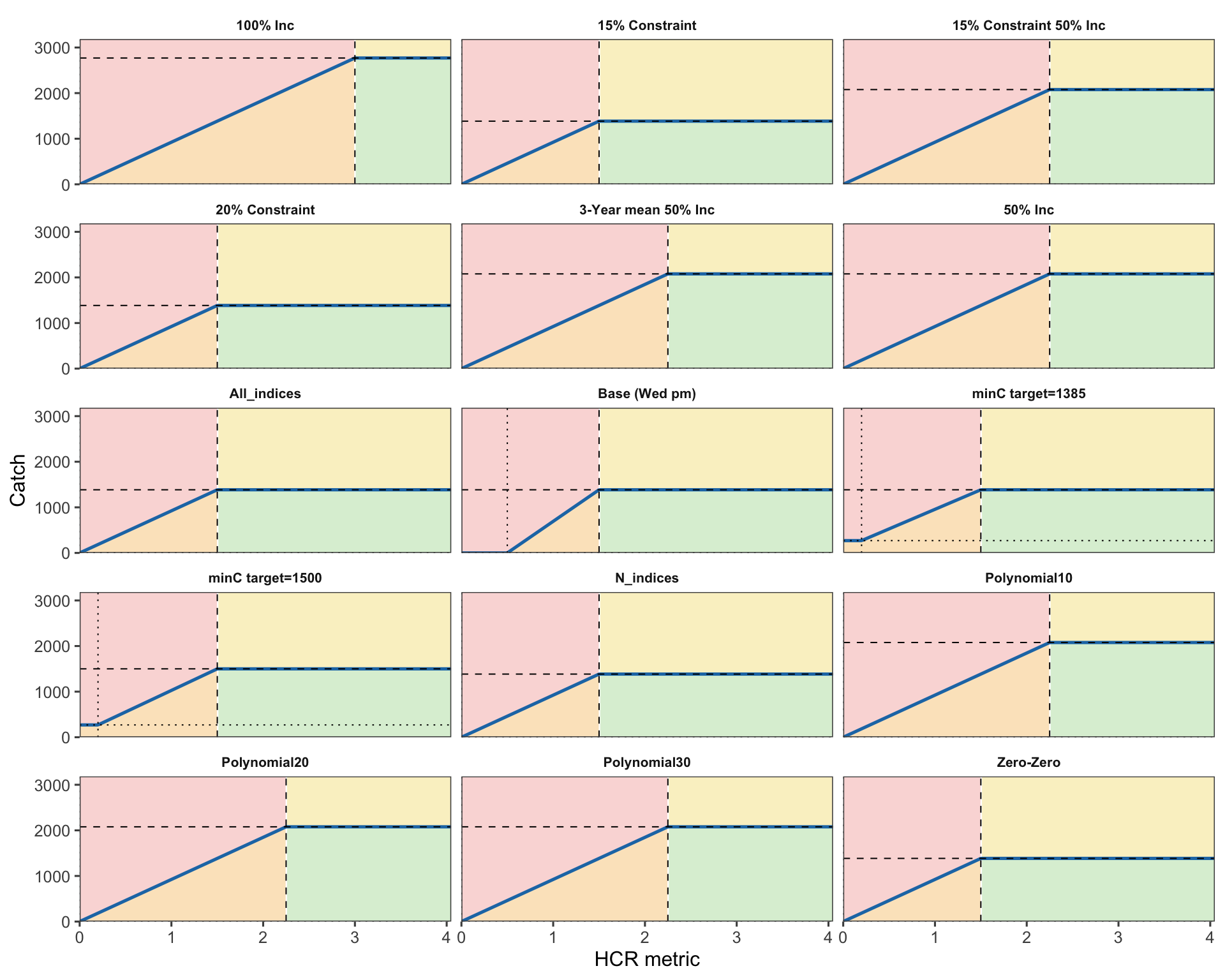
Run these tests from the root of the jmMSE repository. The normal setup route is to source config.R, because it loads the FLR, MSE, and local helper dependencies and sources utilities.R.

# From /path/to/jmMSE
cores <- 3
source("config.R")

The current implementation requires the following R packages directly or through config.R:

Package	Main use in this workflow
TAF	Directory creation and workflow conventions
mse	mpCtrl(), mseCtrl(), mp(), mps(), performance machinery
msemodules	Standard estimator, HCR, and implementation modules
FLasher	Forward projection machinery
FLjjm	Jack mackerel OM/OEM objects and performance statistics
FLCore	FLR data structures used by the OM and index objects
data.table	Tabular setup and summarisation
ggplot2	HCR and diagnostic plotting
future, future.apply, doFuture	Parallel execution

Optional packages are needed only for exploratory diagnostics and smoothing screens:

Package	Use
mgcv	Smooth response-surface diagnostics for parameter screens
akima	Interpolation for contour diagnostics
lhs	Latin-hypercube parameter screens

3 Data and Object Prerequisites

Before running CMP tests, confirm that the conditioned OM files exist and can be loaded. For the current one-stock example, the required file is:

file.exists("data/om11_h1_0.16_065.rds")

The standard loading block is:

cores <- 3
source("config.R")

mkdir("model/indices")

om11 <- readRDS("data/om11_h1_0.16_065.rds")
spread(om11, FORCE = TRUE)

iy <- 2025
fy <- 2050
ty <- seq(iy + 11, iy + 15)
rys <- ac(seq(2019, 2023))

cprop <- catch_props(om)$last5

After spread(om11, FORCE = TRUE), the object components used below are available in the global session as om, oem, and iem.

4 CMP Test Table

Table 1: Candidate CMP tests requested for the index-based hockeystick test set.

CMP name	min	lim	trigger	target	dlow	dupp	smooth	indices	output	status
Base (Wed pm)	0	0.5	1.50	1385.0	unconstrained	unconstrained	4 years	Chile_CPUE, Offshore_CPUE	catch	available
Zero-Zero	0	0.0	1.50	1385.0	unconstrained	unconstrained	4 years	Chile_CPUE, Offshore_CPUE	catch	available
15% Constraint	0	0.0	1.50	1385.0	0.85	1.20	4 years	Chile_CPUE, Offshore_CPUE	catch	available
20% Constraint	0	0.0	1.50	1385.0	0.80	1.20	4 years	Chile_CPUE, Offshore_CPUE	catch	available
50% Inc	0	0.0	2.25	2077.5	unconstrained	unconstrained	4 years	Chile_CPUE, Offshore_CPUE	catch	available
15% Constraint 50% Inc	0	0.0	2.25	2077.5	0.85	1.20	4 years	Chile_CPUE, Offshore_CPUE	catch	available
3-Year mean 50% Inc	0	0.0	2.25	2077.5	0.85	1.20	3 years	Chile_CPUE, Offshore_CPUE	catch	available
Polynomial10	0	0.0	2.25	2077.5	0.85	1.20	poly (enp = 0.1)	Chile_CPUE, Offshore_CPUE	catch	not available as polynomial today
Polynomial20	0	0.0	2.25	2077.5	0.85	1.20	poly (enp = 0.2)	Chile_CPUE, Offshore_CPUE	catch	not available as polynomial today
Polynomial30	0	0.0	2.25	2077.5	0.85	1.20	poly (enp = 0.3)	Chile_CPUE, Offshore_CPUE	catch	not available as polynomial today
100% Inc	0	0.0	3.00	2770.0	0.85	1.20	4 years	Chile_CPUE, Offshore_CPUE	catch	available
minC target=1385	270	0.2	1.50	1385.0	0.85	1.20	4 years	Chile_CPUE, Offshore_CPUE	catch	available
minC target=1500	270	0.2	1.50	1500.0	0.85	1.20	4 years	Chile_CPUE, Offshore_CPUE	catch	available
All_indices	0	0.0	1.50	1385.0	0.85	1.20	4 years	Chile_CPUE, Offshore_CPUE, Chile_AcousN, Peru_Artis	catch	available after index-name check
N_indices	0	0.0	1.50	1385.0	0.85	1.20	4 years	Chile_AcousN, Peru_Artis	catch	available after index-name check

The table uses current jmMSE index names where these differ from the shortened workshop labels:

• C_CPUE means Chile_CPUE.
• offshore means Offshore_CPUE.
• Acoustic_N means Chile_AcousN.
• Peru_Art means Peru_Artis.

5 Availability Notes

The immediately available tests are the hockeystick tests that use combine = "mean" in cpues.ind() and pass HCR arguments to hockeystick.hcr(). These include the base, zero-zero, 15% constraint, 20% constraint, 50% increase, 100% increase, minimum-catch, and three-year mean rows.

The rows labelled Polynomial10, Polynomial20, and Polynomial30 are not available as polynomial tests today. The current jmMSE code has a combine = "smooth" option in cpues.ind(), implemented through smooth_index() and a loess effective-parameter multiplier (enp.mult), not a polynomial smoother. These rows can be run today as loess-smoothed index sensitivity tests with enp.mult = 0.1, 0.2, and 0.3, but they should not be labelled as polynomial CMPs unless a polynomial estimator is added.

The All_indices and N_indices rows should be checked against the exact index names present in the selected OM/OEM before running. Use:

names(observations(oem)$CJM$idx)

If an index name is absent, stop and document the mismatch rather than silently substituting another index.

6 Step-by-Step Implementation

6.1 Step 1: Define the CMP table in R

Use one table as the source of truth for the rows to run. This avoids hand-editing individual control blocks.

cmp_specs <- data.table::data.table(
  cmp = c(
    "Base (Wed pm)",
    "Zero-Zero",
    "15% Constraint",
    "20% Constraint",
    "50% Inc",
    "15% Constraint 50% Inc",
    "3-Year mean 50% Inc",
    "100% Inc",
    "minC target=1385",
    "minC target=1500",
    "All_indices",
    "N_indices"
  ),
  min = c(0, 0, 0, 0, 0, 0, 0, 0, 270, 270, 0, 0),
  lim = c(0.5, 0, 0, 0, 0, 0, 0, 0, 0.2, 0.2, 0, 0),
  trigger = c(1.5, 1.5, 1.5, 1.5, 2.25, 2.25, 2.25, 3.0, 1.5, 1.5, 1.5, 1.5),
  target = c(1385, 1385, 1385, 1385, 2077.5, 2077.5, 2077.5, 2770, 1385, 1500, 1385, 1385),
  dlow = c(NA, NA, 0.85, 0.80, NA, 0.85, 0.85, 0.85, 0.85, 0.85, 0.85, 0.85),
  dupp = c(NA, NA, 1.20, 1.20, NA, 1.20, 1.20, 1.20, 1.20, 1.20, 1.20, 1.20),
  nyears = c(4, 4, 4, 4, 4, 4, 3, 4, 4, 4, 4, 4),
  combine = "mean",
  indices = list(
    c("Chile_CPUE", "Offshore_CPUE"),
    c("Chile_CPUE", "Offshore_CPUE"),
    c("Chile_CPUE", "Offshore_CPUE"),
    c("Chile_CPUE", "Offshore_CPUE"),
    c("Chile_CPUE", "Offshore_CPUE"),
    c("Chile_CPUE", "Offshore_CPUE"),
    c("Chile_CPUE", "Offshore_CPUE"),
    c("Chile_CPUE", "Offshore_CPUE"),
    c("Chile_CPUE", "Offshore_CPUE"),
    c("Chile_CPUE", "Offshore_CPUE"),
    c("Chile_CPUE", "Offshore_CPUE", "Chile_AcousN", "Peru_Artis"),
    c("Chile_AcousN", "Peru_Artis")
  )
)

6.2 Step 2: Add the smoothed sensitivity rows separately

These rows are available only as loess-smoothed sensitivity tests unless a polynomial smoother is implemented.

smooth_specs <- data.table::data.table(
  cmp = c("Polynomial10_as_loess", "Polynomial20_as_loess", "Polynomial30_as_loess"),
  min = 0,
  lim = 0,
  trigger = 2.25,
  target = 2077.5,
  dlow = 0.85,
  dupp = 1.20,
  nyears = 4,
  combine = "smooth",
  enp.mult = c(0.1, 0.2, 0.3),
  indices = list(
    c("Chile_CPUE", "Offshore_CPUE"),
    c("Chile_CPUE", "Offshore_CPUE"),
    c("Chile_CPUE", "Offshore_CPUE")
  )
)

6.3 Step 3: Check index availability

Stop if requested indices are not available in the current OEM.

available_indices <- names(observations(oem)$CJM$idx)

check_indices <- function(indices) {
  missing <- setdiff(indices, available_indices)
  if(length(missing) > 0) {
    stop("Missing requested indices: ", paste(missing, collapse = ", "))
  }
  invisible(TRUE)
}

invisible(lapply(cmp_specs$indices, check_indices))

6.4 Step 4: Build a single CMP control object

This helper converts one CMP table row into an mpCtrl() object. It is the safest way to keep the table and implementation synchronized.

make_cmp_ctrl <- function(spec, om, rys) {
  hcr_args <- list(
    metric = "mean",
    output = "catch",
    target = spec$target,
    min = spec$min,
    lim = spec$lim,
    trigger = spec$trigger,
    initial = 1385
  )

  if(!is.na(spec$dlow)) hcr_args$dlow <- spec$dlow
  if(!is.na(spec$dupp)) hcr_args$dupp <- spec$dupp

  est_args <- list(
    refyrs = rys,
    combine = spec$combine,
    nyears = spec$nyears,
    indices = spec$indices[[1]]
  )

  if("enp.mult" %in% names(spec)) {
    est_args$enp.mult <- spec$enp.mult
  }

  mpCtrl(
    est = mseCtrl(method = cpues.ind, args = est_args),
    hcr = mseCtrl(method = hockeystick.hcr, args = hcr_args),
    isys = mseCtrl(method = split.is, args = list(split = catch_props(om)$last5))
  )
}

6.5 Step 5: Run one example CMP

The 15% constraint row is a useful example because it exercises the normal two-index estimator, the hockeystick HCR, and the interannual catch-change constraints.

example_spec <- cmp_specs[cmp == "15% Constraint"]
example_ctrl <- make_cmp_ctrl(example_spec, om = om, rys = rys)

example_run <- mp(
  om,
  oem = oem,
  iem = iem,
  control = example_ctrl,
  args = list(iy = iy, fy = fy)
)

performance(example_run) <- performance(example_run, statistics = statistics)

performance(example_run)[statistic == "green" & year %in% ty,
  .(green = mean(data)), by = year]

Inspect the HCR decisions and plotted trajectory before launching all rows:

plot_hockeystick.hcr(example_ctrl$hcr)
plot(om, example_run)
inspect(tracking(example_run), "*hcr")

6.6 Step 6: Run all immediately available CMP rows

Parallel execution is appropriate once the single-row example has completed. Use no more workers than available physical cores, and reduce workers if memory pressure is observed.

library(future.apply)

workers <- min(6L, future::availableCores())
plan(multisession, workers = workers)

cmp_runs <- future_lapply(seq_len(nrow(cmp_specs)), function(i) {
  spec <- cmp_specs[i]
  ctrl <- make_cmp_ctrl(spec, om = om, rys = rys)
  out <- mp(
    om,
    oem = oem,
    iem = iem,
    control = ctrl,
    args = list(iy = iy, fy = fy)
  )
  performance(out) <- performance(out, statistics = statistics)
  out
})

names(cmp_runs) <- cmp_specs$cmp

save(cmp_specs, cmp_runs, file = "model/indices/cmp_tests_paper09.rda",
  compress = "xz")

On Linux or macOS, plan(multicore, workers = workers) may be faster. Use multisession if forked processing is unstable or if running on Windows.

6.7 Step 7: Summarise tuning-period performance

Use the same tuning years across rows. The current working convention is 2036:2040, defined as iy + 11 through iy + 15.

cmp_perf <- performance(cmp_runs, statistics = statistics)

cmp_summary <- periodsPerformance(cmp_perf, list(tuning = ty))

plotBPs(cmp_summary, statistics = c("C", "green", "IACC", "SB"))
plotTOs(cmp_summary, x = "C", y = c("green", "IACC", "SB"))

green_summary <- cmp_perf[statistic == "green" & year %in% ty,
  .(green = mean(data)), by = .(run, year)]

green_period <- green_summary[, .(green = mean(green)), by = run][order(-green)]
green_period

6.8 Step 8: Run smoothed sensitivity rows only if labelled correctly

Do not report these as polynomial tests unless a polynomial estimator is implemented. For now, the following runs are loess-smoothed index sensitivity tests.

smooth_runs <- future_lapply(seq_len(nrow(smooth_specs)), function(i) {
  spec <- smooth_specs[i]
  check_indices(spec$indices[[1]])
  ctrl <- make_cmp_ctrl(spec, om = om, rys = rys)
  out <- mp(
    om,
    oem = oem,
    iem = iem,
    control = ctrl,
    args = list(iy = iy, fy = fy)
  )
  performance(out) <- performance(out, statistics = statistics)
  out
})

names(smooth_runs) <- smooth_specs$cmp

save(smooth_specs, smooth_runs,
  file = "model/indices/cmp_smooth_sensitivity_paper09.rda",
  compress = "xz")

7 Approximate Run Time

Run time depends mostly on the number of OM iterations, projection years, number of stocks, and number of workers. The following planning values are intended for workshop scheduling rather than benchmarking:

Task	Expected time
Load OM and source config.R	Less than 1 minute if packages are installed
One CMP row with about 100 iterations	A few minutes
One CMP row with about 1,000 iterations	Often 10–30 minutes, depending on machine and OM complexity
12 immediately available rows at 100 iterations with 4–6 workers	Roughly 15–45 minutes
12 rows at full iteration count	Potentially several hours
Smooth-index sensitivity rows	Similar to standard rows, with additional estimator overhead

For same-day workshop testing, first run the example CMP with a reduced iteration subset. Then run all available rows with the same reduced subset to detect coding errors and obvious performance differences. Only after the reduced run is stable should the full iteration set be launched.

8 Quality-Control Checklist

Before presenting results, check:

1. The requested indices are present in the selected OEM.
2. The reported CMP labels match the actual estimator and HCR arguments used.
3. The polynomial rows are either renamed as loess-smoothed sensitivity rows or held back.
4. The tuning years are consistent across all rows.
5. green, C, IACC, and SB are computed from the same saved run object.
6. The saved .rda output contains both the CMP table and run object, so each result is traceable to the row that produced it.
7. Figures in the workshop report cite the source file, date, OM, iteration count, and whether results are reduced-iteration or full-iteration runs.

9 Recommended Same-Day Test Order

1. Run Zero-Zero as the basic unconstrained hockeystick control.
2. Run 15% Constraint and 20% Constraint to verify interannual catch-change caps.
3. Run 50% Inc and 15% Constraint 50% Inc to evaluate the higher target/trigger pair.
4. Run minC target=1385 to verify the minimum-catch floor.
5. Run All_indices and N_indices only after index-name checks pass.
6. Hold Polynomial10, Polynomial20, and Polynomial30 unless they are explicitly relabelled as loess-smoothed sensitivity tests.