SC13 - JM09 Report of the Management Strategy Evaluation (MSE) workshop (SCW15), July 14-18, 2025
Published
2025-08-24
1 Summary
The Jack Mackerel Management Strategy Evaluation (MSE) Technical Workshop brought together scientists, technical experts, and external reviewers to assess recent progress and refine the MSE framework being developed under South Pacific Regional Fisheries Management Organisation (SPRFMO). The primary goal of the workshop was to ensure that the modeling framework is scientifically sound, technically robust and transparent, and to produce a set of candidate management procedures to present to the 13th SC, as outlined by the Commission (e.g., SPRFMO Jack Mackerel Working Group (2025)). The workshop was successful in testing the framework, it resulted in improved understanding of scientists in its functioning and ability to test alternative MPs. Discussions during the workshop contributed to some changes made in the conditioning of the Operating Models (OMs) and in the algorithms of the harvest control rules to improve the robustness of the results. Further review and discussion are needed to agree on a set of candidate management procedures. Finally, the framework and preliminary results were accepted by the group as the basis for recommendations to the Science Committee.
Key Outcomes and Advancements
MSE Framework Consolidation
Participants reviewed the jmMSE software package, confirming that it provides a robust and flexible platform for conducting MSEs. The package includes 1) a reference set of operating models conditioned to historical data using Markov Chain Monte Carlo (MCMC; an efficient MP tuning algorithm), and 2) tools for visualizing and comparing results.
MSE and OM Fine-Tuning
The workshop focused on refining the operating models (OMs) to ensure they accurately represent the jack mackerel stock dynamics and future behaviour. Participants discussed and implemented changes to the OM structure, including adjustments to recruitment dynamics and selectivity patterns. These refinements were aimed at improving the realism of the OMs and their ability to simulate plausible future scenarios.
Robustness Testing
The workshop clarified the role and scope of robustness tests. These tests are intended to explore how candidate MPs perform under a range of plausible yet uncertain scenarios rather than represent definitive alternative models. Scenarios reflecting changes in recruitment, spatial availability, environmental regime shifts (e.g., El Niño Southern Oscillation (ENSO)), and stock structure were reviewed and refined for implementation.
Indicator-driven MPs and harvest control rule (HCR) logic
The workshop evaluated empirical MPs based on one or more indicators, with focus on two formulations:
Total Allowable Catch (TAC) as a product of a target and a multiplier from an index (e.g. biomass from scientific surveys and /or commercial catch per unit effort (CPUE)).
TAC adjusted incrementally from the previous year based on index signals.
The workshop tuned the MPs using the probability of being in the green zone of a Kobe plot (i.e., the biomass level is above the \(B_{MSY}\) and the fishing effort is below \(F_{MSY}\)) as an objective. All candidate MPs were tuned to achieve a probability value of 60%, a value identified using a questionaire distributed to members during COMM13.
Recommendations and refinements
The participants recommended additional diagnostics and refinements, including:
Adding plots of how index trajectories relate to TACs.
New performance metrics that reflect stock status and trends in the final projection years.
Ensuring consistent treatment of selectivity, weights-at-age, and catch splits in both projections and reference point calculations.
Exploring robustness scenarios that account for variability in fleet selectivity and biological assumptions, particularly where CPUE is used as an input.
Exploring alternative HCRs.
Documentation and transparency
The participants emphasized the importance of transparency in documenting model assumptions, data sources, and MP structure. The group agreed on priorities for improving documentation and sharing annotated examples of MP behavior.
Next steps and implementation
The next phase of this work will focus on finalizing the candidate MPs, running the robustness tests, and summarizing trade-offs across key performance indicators. In discussions, we also identified future reporting needs, including summary tables and figures for managers, and exploration of reference points and evaluation criteria beyond the green zone probability.
–>
–>
2 Workshop introduction
Management Strategy Evaluation (MSE) has emerged as a critical tool for fisheries management, especially in contexts where data are limited or uncertainty is high. Foundational software frameworks like FLR were developed to facilitate reproducible, cross-disciplinary evaluation of management strategies through simulation and decision analysis (Kell et al. 2007). Building on this foundation, recent advances have expanded FLR’s capacity for data-rich and data-limited systems alike, improving accessibility and integration with other tools (Hillary et al. 2023). Complementing these developments, a structured framework for evaluating methods and risk in data-limited fisheries has been proposed, providing practical guidance on the application of MSE in real-world settings (Carruthers et al. 2023).
The SCW15 Jack Mackerel MSE Technical Workshop was convened in response to the Scientific Committee’s request for progress on developing and evaluating MPs for jack mackerel under the SPRFMO framework. The meeting was held over five days (14–18 July 2025) and hosted in a hybrid format, with active participation from in-person attendees in Seattle and remote collaborators from SPRFMO Member States and invited experts. This event built on previous technical work, including the SCW14 benchmark. The focus was on finalizing the reference set of OMs, implementing robustness tests, and refining candidate MPs using the jmMSE software package.
Throughout the week, participants engaged in live coding sessions, software validation, model tuning, and scenario refinement. The agenda was intentionally flexible, allowing the group to respond dynamically to technical challenges as they emerged. Examples of these included issues with index generation, selectivity patterns, and catch variability under different MP formulations. The workshop emphasized transparency, reproducibility, and documentation, with clear objectives to improve the utility and credibility of the MSE outputs ahead of Scientific Committee and Commission review.
The appendices provide the participants, the agenda, and the daily summary activities in the workshop minutes. A summary review written by the external experts is also provided here.
The following sections review the work conducted during the workshop, separated into three sections: 1) reviewing the OM specifications, 2) implementing robustness tests, and 3) applying and refining of candidate MPs. We conclude with a set of recommendations for the SC to consider.
3 Review of the Operating Model specifications
The workshop reviewed the current specifications of the OMs. In particular, the assumptions for the reference point calculations were discusssed and contrasted with the 2024 assessment results and reports (South Pacific Regional Fisheries Management Organisation (2024)). Due to the terminal (2024) estimates of fisheries selectivities, the assessment report had anomalously high values for \(F_{MSY}\)
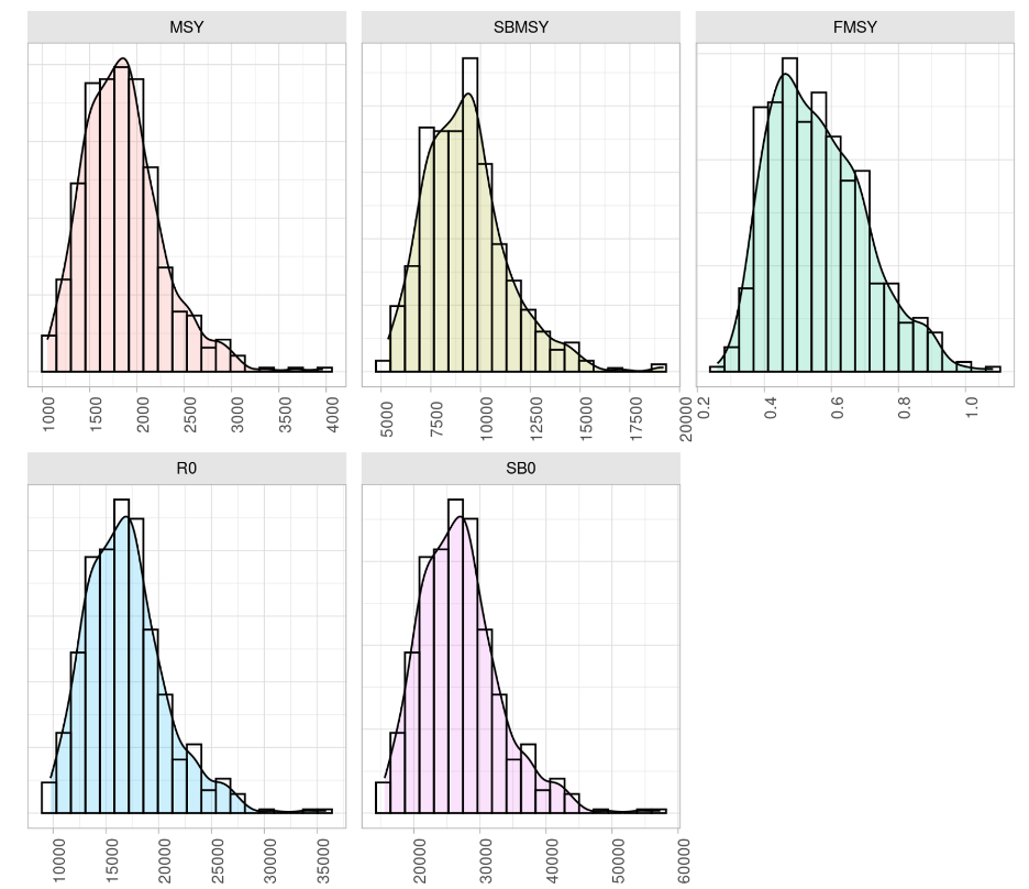
While the 2024 stock assessment produced high estimates of potential catch under the third tier of the harvest control rule—exceeding 4,900 kt based on \(F_{MSY}\)—this result was considered unrealistic under current fleet capacities. That was due to likely upward bias in \(F_{{MSY}}\) estimates caused by strong selection on older fish. As a result, the Scientific Committee recommended constraining the 2025 TAC to be at or below 1,428 kt, representing only a 15% increase from 2024 levels and aligned with the Commission’s guidance. In developing the OM, reference points such as \(F_{{MSY}}\) were instead based on longer-term averages in fishery selectivity estimates to avoid the influence of short-term variability or cohort effects, ensuring more stable and precautionary management advice consistent with the MSE framework (Figure 1).
Figure 1: Distribution of reference points from the operating model discussed during the workshop.
Some issues were identified with the current stock assessment that warrant further attention ahead of the next benchmark. Among them are assumptions about mean body weight at age (specifically in the last year with incomplete data). The Scientific Committee emphasized the need for standardizing CPUE indices and improving data collection protocols, particularly regarding fleet-specific efficiency changes. Sensitivities to early age composition data—especially from the pre-1990 period—remain unresolved, with residual patterns noted for the North Chilean fleet. In addition, assumptions underlying selectivity and recruitment regimes were highlighted as critical sources of uncertainty, with substantial influence on reference points and management advice. Finally, the participants underscored the importance of continued evaluation of single-stock versus two-stock model structures using simulation and MSE tools.
4 OM scenarios for robustness testing
4.1 Simulating El Niño effects in the Operating Model
To incorporate climate-driven variability into the Operating Model (OM) projections, we defined a scenario simulating El Niño–like events every five years beginning in 2030. These events affect primarily recruitment and distribution options. Based on the work of Iago and available literature, we proposed an initial set of biological and fishery processes that most likely relate to El Niño conditions. The group discussed these and noted that others may be best considered in the next round of stock assessment benchmark and for future MSE work.
The table below summarizes the proposed effects of simulated El Niño conditions on the OM, categorizing them by their expected direction, biological or fishery-based justification, and evaluation priority. The table is divided into two sections: effects that are prioritized for immediate evaluation and those deferred for further study.
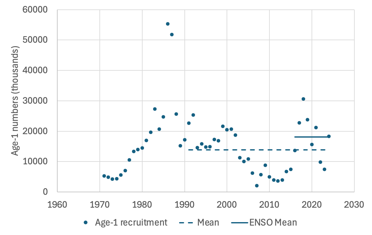
The first section highlights two key El Niño-driven effects: 1) a 30% increase in recruitment with a one-year lag, linked to ENSO-related early life stage survival (Figure 2), and 2) shifts in catchability, with coastal regions experiencing increased availability and offshore regions seeing declines, reflecting observed onshore movement of fish during warm anomalies. The latter effect was identified as high-priority, with a focus on quantifying impacts on fishery removals.
The deferred effects included the potential for reduced weight-at-age (potentially due to prey scarcity), earlier maturity (a stress response observed in small pelagics), and increased natural mortality (from predation or environmental stress). These are flagged for future study, pending historical data checks or further evidence. The table succinctly organizes hypotheses while clarifying immediate next steps for the OM framework.
Figure 2: Recruitment estimates and mean values (horizontal lines) used to estimate the impact of ENSO effects.
The following tables summarizes the key effects, their expected directions, and justification.
Effect
Direction
Justification
Recruitment ↑20%
↑ 1-year lag
ENSO-linked early life stage effects on recruitment
Regional availability
Coast catchability ↑ and offshore ↓
Onshore shift during warm anomalies
Discussed but deferred for further study
Effect
Direction
Justification
Notes
Weight-at-age
↓Productivity
Lower prey density and observed condition declines
Check historical WAA anomalies
Age-1 maturity
Earlier maturity
Stress response seen in small pelagics
similar impact on Recruitment
Coastal selectivity
Age 1–2 sel ↑
Spatial contraction, availability change
Confirm from CPUE by age?
M ↑30%/20%
↓ Survival
Stress-induced mortality, predation
Estimating relative availability from catch proportions
To estimate the relative availability of jack mackerel to different fleets, we analyzed catch proportion data from 2004 to 2024. These data were smoothed using a 5-year moving average to reduce annual variability. The data from the Chilean, Peruvian, and Ecuadorian fleets were classified as coastal, whereas the data from the other fleets were classified as “offshore” for the purpose of approximating changes in avaialbility. The goal was to have some basis for defining changes in availability to coastal and offshore areas in a way that could roughly approximate the effective catchability \(q\) (which includes both true catchability and availability) of the fishery for each fleet, i.e.:
Thus, observed catch proportions can serve as a proxy for relative availability of the resource to each fleet.
5-year moving averages of the proportion of the catch occurring in the “coastal” areas compared to the offshore fleet.
Year Range
Coastal (%)
Offshore (%)
2004–2008
81
19
2005–2009
78
22
2006–2010
74
26
2007–2011
76
24
2008–2012
78
22
2009–2013
82
18
2010–2014
84
16
2011–2015
86
14
2012–2016
86
14
2013–2017
85
15
2014–2018
86
14
2015–2019
87
13
2016–2020
91
9
2017–2021
93
7
2018–2022
94
6
2019–2023
94
6
2020–2024
94
6
Mean
85
15
Range of changes in estimated availability
Given the shift in catch proportions over this period, we can assume a relative catchability due to an environmental effect. We note that the coastal effective catchability increased from a low of 74% (2006–2010) to a high of 94% (2018–2024), representing 20 percentage point change. Meanwhile, the offshore effective catchability declined from a high of 26% (2006–2010) to a low of 6% (2018–2024), representing a decrease of 20%.
As part of the robustness test, we propose that the effective availability to the offshore fleet gradually drops from 15% of the mean biomass to 6% during El Niño periods (a 60% decline in \(q\) ). This would apply to the data generated for offshore CPUE index in the simulations. For the coastal zones, the effect of El Niño would correspond to an 11% increase in the availability of fish relative to the mean (85%). These changes would apply to the Chilean south-central CPUE index and the Peruvian CPUE index data generation. This is one proposal among many that could be imagined. For example, a slightly more conservative range could be based on the 10th and 90th percentiles of estimated effective catchability (from proportional catches):
These shifts may provide some scope for showing the impact of changes in the relative abundance indicators in index values. These reflect patterns over the past two decades, possibly due to environmental changes.
5 Management Procedure formulation and tuning
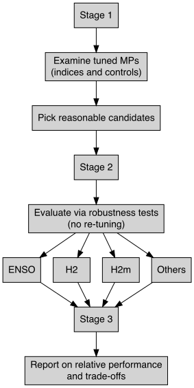
We provide a general outline for the workflow for defining and evaluating MPs, dividing the process into three main stages (Figure 3). The framework for this workflow was made available to all participants to explore and implement.
Figure 3: Workflow for evaluating and selecting candidate management procedures (MPs).
5.1 Tuning to P(Green)
In Stage 1, a key activity is to “tune” MPs towards a common objective. Tuning MPs allows for more direct and straightforward comparisons of trade-offs between candidate MPs. The tuning objective was set as the probability of being in the green zone of the Kobe plot (i.e., the biomass level is above the \(B_{MSY}\) and the fishing effort is below \(F_{MSY}\)) for the final years of the projection period. This probability is denoted as (“P(Green)”). All candidate MPs were tuned to achieve a P(Green) value of 60%, a value identified using a questionaire distributed to members during COMM13.
During the tuning process, the group noted that the current high stock status tended to increase catch levels, particularly at the beginning of the projection period. This can result in declining stock trends later in the projection period, even when the short-term performance criteria are met, since the current P(Green) is well above this 60% target. There were also difficulties ascertaining how the projected TACs were calculated from the empirical MPs that were being tested.
We also tuned MPs using short-cut assessment methods, mimicking the behaviour of the jjm model as used by the Jack Mackerel Working Group (JMWG) for advisory purposes. These short-cut approaches considered observations with relatively low uncertainty, high uncertainty and uncertainty with autocorrelation incorporated. Results using these short-cuts can be found in @Section 8.2.
6 Summary of Workshop Outcomes
The SCW15 workshop provided a venue for progressing the Jack Mackerel MSE work, resolving some technical issues, and evaluating multiple MP configurations. A key outcome was the identification of problems in being able to clearly show how a tested MP would perform in terms of reaction to different signals from the indices, and how this would translate into catch levels. The group noted that the current jmMSE framework was capable of simulating a wide range of MPs, but more work is needed for member scientists to effectively communicate the tradeoffs and applicaitons of these MPs to the Commission. The group noted that these issues can be discussed prior to the SC and some technical communications would be encouraged. These have focussed on narrowing MP options and refining things for presentation to the SC. Depending on this direction, it may mean that an additional in-person meeting should occur after February 2026 and the Commission meeting.
Regarding the ability and facility for member scientists to use and evaluate the MSE framework, the group noted that the development of the jmMSE package was exceptionally well done. We found that difficulties inherent to the jack mackerel resource and assessment created unique problems. Specifically, the variable resource distribution, available data, and specifications of projection conditions (e.g., mean body mass-at-age, fishery selectivity at age) complicated how MPs could be evaluated. We noted that such specifications would be problematic for any other MSE framework as well.
Software and Technical Recommendations
Continue using FLR as the main MSE engine unless there is a dedicated effort to migrate to openMSE or another platform.
Improve naming conventions in code to reduce ambiguity. For example:
Functions like cpuescore2.ind and cpuescore3.ind could better reflect their purpose.
Include the current harvest control rule (Annex K modified) and alternative HCRs.
MSE Development Timeline and Deliverables
The group noted that MSE funding (in the form of providing support from external developers) may be available but would be contingent on:
Coordination with the current analyst (Iago).
Collaboration with the technical team.
Receptiveness to using openMSE.
Clear timelines and deliverables.
An initial set of deliverables that have been completed include:
Reference OMs (no multistock): End of July
Robustness OMs (no multistock): End of August progress)*
Shortcut calibration to the JJM assessment: End of August
Range of shortcut MPs run for all reference OMs: End of July
Technical documentation and reports:
Draft Technical Summary Document (TSD) by end of July.
Technical working papers and presentations for:
Shortcut calibration to JJM
Reference set OM results for MP archetypes (pending)
Robustness OM results
MP performance summaries
Slick MSE results summary.
Near term tasks
Participants were encouraged to document their activities during the workshop, including the methods explored and tuning targets used. Work tasked identified included:
All continue to evaluate MPs to the extent practical ensuring that they can be tuned to achieve a 60% green status and are consistent with the available OM data stream projections.
Jim evaluated 9 MPs (including bufferdelta2, cpuescore2, test acoustic, and combinations of CPUE indices with different delta_TAC values), all tuned to achieve 60% green status.
Chilean analysts apply shortcut tuning methods as a demonstration. This was completed and provided in Section 8.2.
This table illustrates how an array of MPs might be evaluated for summarization:
Harvest Control Rule Methods Summary
Comparison of methods, tuning, and compatibility
Year
Method
Metric
Tuning Parameter
Other Parameters
Score Index
Comments
2024+
buffer.hcr
depletion
target
bufflow, buffup, limit
cpuescore3.ind
Original pkg function
2024+
bufferdelta.hcr
depletion
width
sloperatio
cpuescore3.ind
Modified; not compatible with z-score metrics
2024+
bufferdelta2.hcr
zscore
width
sloperatio
cpuescore2.ind
New; not compatible with depletion
2024+
buffer2.hcr
zscore
target
width (affects buffer)
cpuescore2.ind
Original; adjusted for zscore (limit = -2 SD)
Summary of MPs evaluated during the workshop, including tuning targets and performance metrics.
Medium term tasks
The group agreed to continue working on the MSE framework, with a focus on the following tasks:
Consider how reference set of OMs could be regenerated conditioned to historical data using MCMC methods.
Implement robustness tests to evaluate how MPs perform under a range of plausible yet uncertain scenarios.
Refine MP candidates using the jmMSE software package, ensuring they are scientifically sound and technically robust and transparent.
Document and share the MSE framework, including model assumptions, data sources, and MP structure.
Explore additional diagnostics and refinements, including new performance metrics that reflect stock status and trends in the final projection years.
6.1 Further recommendations to consider
For the SC:
Adopt the current proposal structure (timeline and deliverables) with flexibility for future adjustment.
Continue the review process to identify a shortlist of MP options to simplify the selection process at the Commission level.
Consider a placeholder method for calculating the 2026 TAC since MSE work requires further development.
For Members:
Commit to a shared MSE software base (FLR or openMSE).
Engage in pre-SC online meetings to broaden participation in MSE discussions.
For Analyst (Iago):
Prioritize enhancements discussed during the workshop:
Code clarity and naming conventions
Logical parameter usage across MPs
Refinement of FLR-to-dataframe functions
Identify successor strategy after contract ends in 2025.
Carruthers, Thomas R., Quang C. Huynh, Adrian R. Hordyk, David Newman, Anthony D. M. Smith, Keith J. Sainsbury, Kevin Stokes, et al. 2023. “Method Evaluation and Risk Assessment: A Framework for Evaluating Management Strategies for Data-Limited Fisheries.”Fish and Fisheries 24 (6): 1335–50. https://doi.org/10.1111/faf.12726.
Hillary, Richard M., José M. Castro, James T. Thorson, Sean C. Anderson, and Laurence T. Kell. 2023. “The FLR Software Framework for Building Management Strategy Evaluation Systems: Recent Advances and Application to Data-Rich and Data-Limited Fisheries.”Fisheries Research 263: 106585. https://doi.org/10.1016/j.fishres.2023.106585.
Kell, Laurence T., Iago Mosqueira, Paul Grosjean, Jean-Marc Fromentin, Dorleta Garcia, Richard Hillary, Ernesto Jardim Simon Mardle, et al. 2007. “FLR: An Open-Source Framework for the Evaluation and Development of Management Strategies.”ICES Journal of Marine Science 64 (4): 640–46. https://doi.org/10.1093/icesjms/fsm012.
The following sections document some of the work undertaken by workshop participants during and after the workshop.
8.1 Package development
The SC Chair, Ricardo, developed some enhancements to the jmMSE demo framework after the workshop. These introduce greater flexibility and diagnostic power through two key components: performance2() and evaluate_mp().
The performance2() function extends standard summary outputs by computing a richer set of indicators. These indicators include mean relative biomass and fishing mortality, catch, the probability of remaining in the green zone of the Kobe plot, and the longest duration spent outside it.
The evaluate_mp() function wraps the full MP simulation while allowing multi-parameter optimization of Harvest Control Rule (HCR) settings. It also incorporates a customizable objective function that accounts for discounted catch, stability (via interannual catch variability (IACV)), conservation thresholds (e.g., probability of being “green”), and duration outside target reference points. This setup allows for filtering out of implausible simulations, facilitates adaptive MP tuning, and supports rapid exploration of trade-offs in management performance. Together, these tools make the MSE evaluation process more transparent, efficient, and tailored to decision-maker priorities.
This and other work conducted after the workshop encountered problems with the magnitude of recruitment variability which led to unreasonably high levels of biomass in a significant number of the simulations. This was something that required further investigation and resolution in collaboration with the developer (Iago).
8.2 Examples of Shortcut MPs
This section was compiled by Ignacio Payá and colleagues from Chile. It summarizes an example implementation of “shortcut” management procedures (MPs) that simplify the estimation and harvest control rule (HCR) steps using buffered depletion-based control. It also illustrates how FLR-based tools can be used to define control logic, evaluate HCR targets, and visualize results using the Slick (Blue Matter Science (2024)) and mseviz (Mosqueira (2022)) R packages for performance evaluation. Each section below includes code, explanation, and figures that demonstrate specific aspects of the approach.
Shortcut MP Definition
This section defines the MP structure using mpCtrl() with shortcut estimation (shortcut.sa), a buffer-based HCR, and a split implementation system (ISYS). Deviations are defined using a lognormal AR(1) process.
HCR Target Exploration
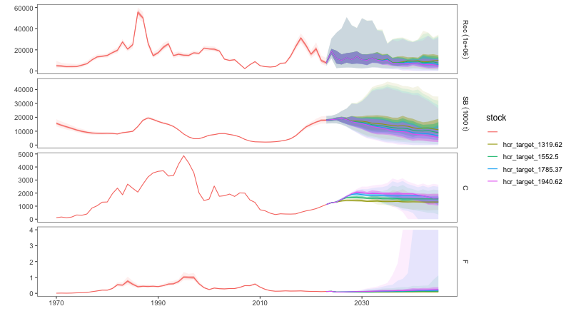
To evaluate MP performance under various Total Allowable Catch (TAC) values, the control object (ctrl) from Section 8.2.1 is tested across a set of TAC multipliers. The target range brackets the 2025 CMM level. In this example, the multipliers tested are 0.85, 1, 1.15, and 1.25 of the 2025 TAC. This produces comparative projection plots for four candidate TAC levels (Figure 4).
Figure 4: Projections for TAC 2025 scenarios using buffer HCR.
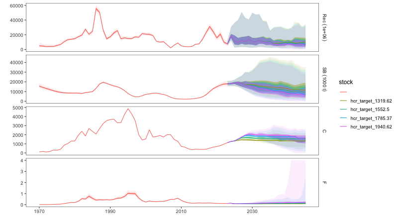
Now we test this with a simple limit on the annual change in TAC, which is a common requirement in many fisheries management systems. In other words, the TAC for a subsequent year cannot increase or decrease beyond a specified percentage. These results compare similarly to those without any TAC constraint (Figure 5). A clearer evaluation of these two sets is shown in the next section using the Slick package.
Figure 5: Projections for TAC 2025 scenarios using buffer HCR with TAC change limit at 15 percent.
Projections for TAC 2025 scenarios using buffer HCR with TAC change limit at 25% (downward) and 15% increases.
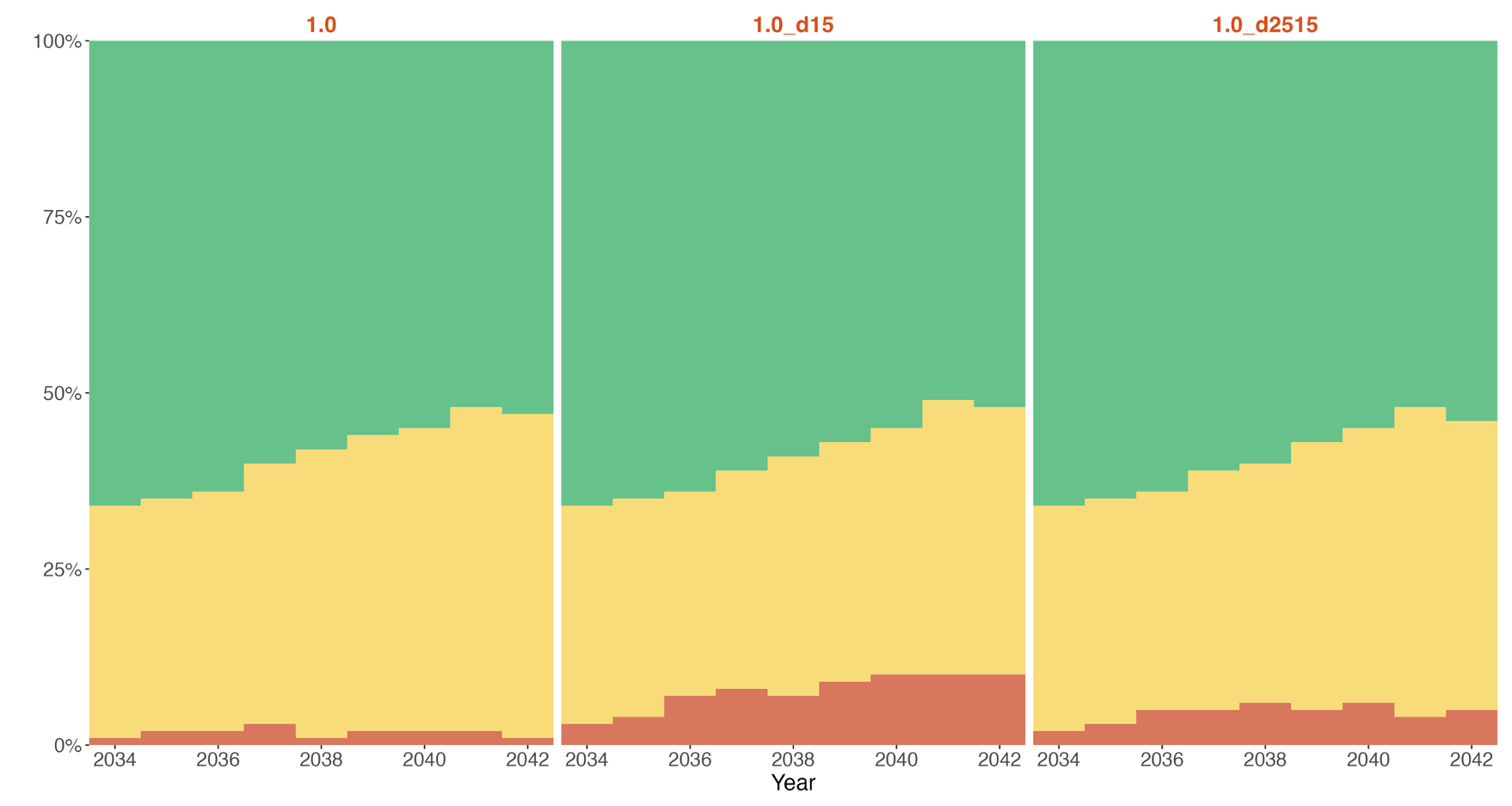
Using the Slick package (Blue Matter Science (2024)), performance metrics such as catch, fishing mortality, and spawning biomass can be summarized across operating models and MPs. As one illustration of the application, we presents a Kobe-style status time series from Slick. We compare three shortcut management procedures (MPs) all tuned to the 2025 TAC level (1.55 million t) but differing in constraints on interannual TAC changes (Figure 6). The panels from left to right represent: (1) no constraint (1.0), (2) symmetric ±15% TAC change limit (1.0_d15), and (3) asymmetric −25%/+15% limit (1.0_d2515). Each panel shows the proportion of simulations over time falling into the green (safe), yellow (overfished or overfishing), and red (overfished and overfishing) zones. While all three MPs maintain a majority of simulations in the green zone, applying TAC constraints leads to a slight increase in the proportion of years falling into the red zone—particularly under the asymmetric constraint. This reflects the trade-off where increased catch stability may slightly elevate biological risk under certain scenarios. We provide a copy of the slick file on the repository under MS Teams at [tbd].
Figure 6: Shortcut application tuned to the 2025 TAC (1,552,500 t) but with different constraints on TAC changes. Left most is no constraint, middle is 15% increase and decrease, right-most is 25% decrease and 15% increase.
Further performance evaluation of the shortcut MPs
This section summarizes performance using FLR tools from the mseviz package (Mosqueira (2022)). Average values are computed for specified periods and used in BRP (Biological Reference Point) and tradeoff plots.
perf <-readPerformance("demo/performance.dat.gz") perf <- perf |>mutate(data=ifelse((statistic=='F'&data>2),2,data))#unique(perf$statistic)perf<- perf %>%mutate(# Extract the part after "_d" and before "_hcr"d_part =str_extract(mp, "(?<=_d)[^_]+"),# Extract the trailing number after the last "_"target_num =str_extract(mp, "[0-9.]+$"),# Create short name by combining themmp =paste0("d", d_part, "_", ifelse(target_num==1319.62,"0.85",ifelse(target_num==1552.5,"1.0",ifelse(target_num==1785.37,"1.15","1.25")))) )perf <-periodsPerformance(perf, periods) # perf |> filter(period=='tuning', statistic %in% c("SB","C", "IACC"), mp %in% c("d00_1.0", "d15_1.0", "d2515_1.0")) |># ggplot(aes(x=as.factor(mp),y=data,fill=mp)) + geom_boxplot(outlier.shape=NA) + ggthemes::theme_few() +# facet_wrap(.~statistic, scales="free_y") png("images/sc_delta_TAC.png", width=900, height=800)plotBPs(perf |>filter(period=='tuning', mp %in%c("d00_1.0", "d15_1.0", "d2515_1.0" )), statistics=c("C","IACC","F","PTAClimit","SB" )) +ggtitle("Shortcut MPs for Tuning Period (2034–2045)") + ggthemes::theme_few(base_size =16) +theme(axis.text.x =element_text(angle =45, hjust =1)) +scale_fill_flr() +ylim(c(0,NA)) +xlab("MP")dev.off()png("images/sc_targ_TAC.png", width=900, height=800)plotBPs(perf |>filter(period=='tuning', mp %in%c("d00_0.85", "d00_1.0", "d00_1.15", "d00_1.25" )), statistics=c("C","IACC","F","SB" )) +ggtitle("Shortcut MPs for Tuning Period (2034–2045)") + ggthemes::theme_few(base_size =16) +theme(axis.text.x =element_text(angle =45, hjust =1)) +scale_fill_flr() +ylim(c(0,NA)) +xlab("MP")dev.off()
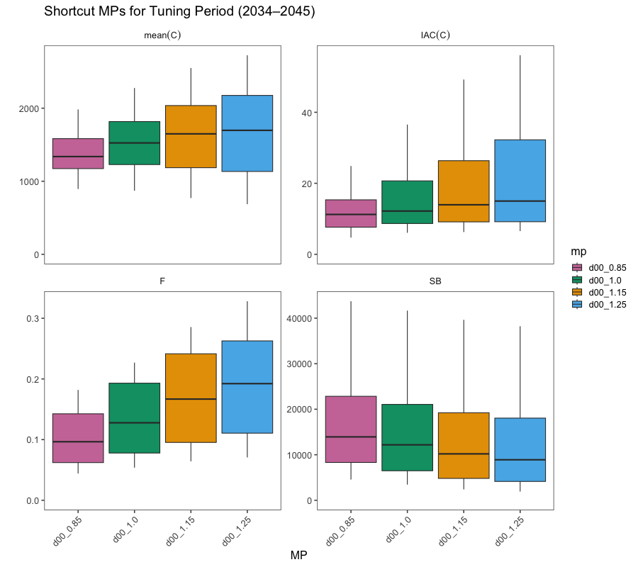
The performance of multiple shortcut MPs over the tuning period (2034–2045) were contrasted as an example. Here, each MP was run with catch “targets” at different level relative to the 2025 TAC (1.5525 million t). They ranged from 85% (d00_0.85) to 125% (d00_1.25), with no constraints on interannual TAC changes. As expected, higher catch targets result in greater average catches (mean(C)), but also increased interannual variability (IAC(C)), as well as higher fishing mortality (F) (Figure 7). Conversely, spawning biomass (SB) declines with increasing catch target, suggesting a clear trade-off between yield and stock conservation. While d00_1.0 balances moderate catch with more stable biomass and fishing pressure, higher targets (d00_1.15 and d00_1.25) achieve larger catches at the cost of reduced SB and greater volatility—highlighting the importance of considering both yield and stability objectives when selecting candidate MPs.
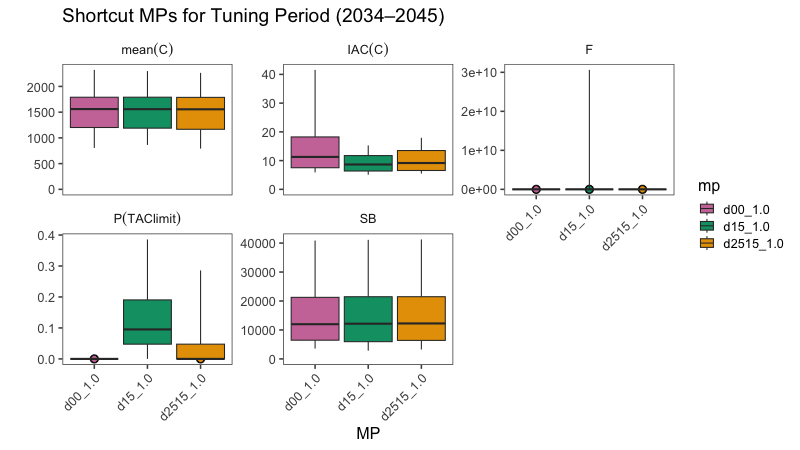
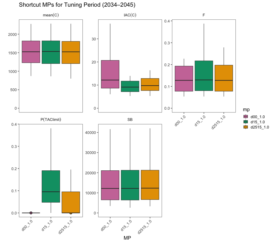
We then compared performance of shortcut MPs all tuned to the 2025 TAC target (1.5525 million t), but with different constraints on interannual changes in TAC. These included (as in the previous figure) no constraint on TAC changes (d00), a symmetric ±15% constraint (d15), and an asymmetric −25%/+15% constraint (d2515). While mean(C) is similar across all three MPs, the application of TAC constraints notably reduces IAC(C) compared to the unconstrained case (Figure 8). This stability comes with trade-offs—particularly a modest increase in the probability of hitting a predefined TAC floor (P(TAClimit)) for d15 and d2515. SB and F remain broadly similar across scenarios, suggesting that moderate TAC constraints can improve catch stability without severely compromising stock status. Overall, the results highlight the stabilizing benefit of delta-TAC constraints, with d15 offering the most consistent balance of catch, stability, and conservation performance.
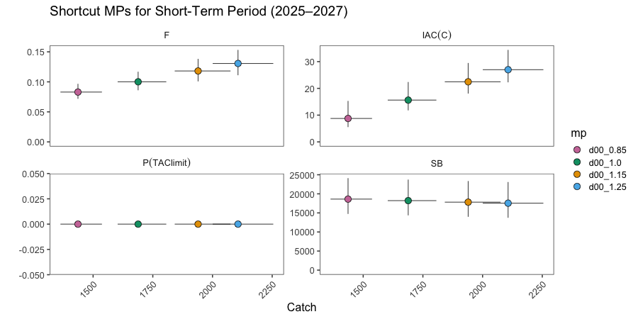
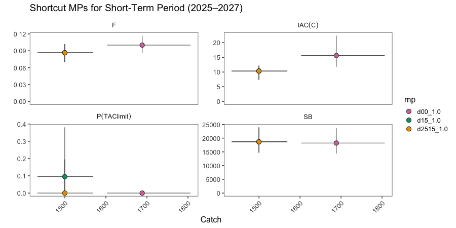
As an alternative, we show figures that highlight short-term (2025–2027) trade-offs among shortcut MPs based on either different TAC targets (Figure 9) or different TAC change constraints (Figure 10). Increasing the TAC target from 85% to 125% of the 2025 TAC results in expected increases in catch, but also in F and IAC(C), with slight declines in spawning SB. All options show negligible P(TAClimit). In contrast, comparing MPs with the same TAC target (2025 level) but different delta-TAC constraints (Figure 10). While d00_1.0 provides slightly higher short-term catch, it exhibits greater catch variability and a marginally higher risk of triggering the TAC limit compared to d15_1.0 and d2515_1.0. These results suggest that in the short term, applying TAC constraints can enhance stability and reduce the risk of severe TAC cuts, albeit in catch—highlighting a management choice between maximizing short-term yield and reducing volatility.
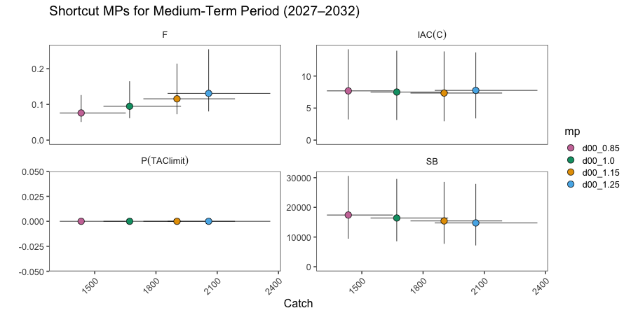
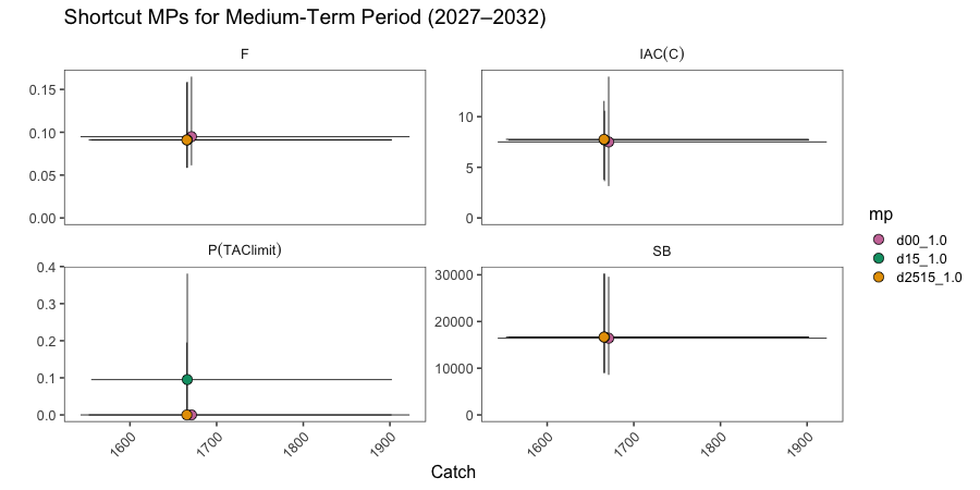
While the general patterns observed in the short-term persist, the medium-term results show reduced separation across MPs in all performance metrics. For instance, in the TAC target comparison (top panel), differences in F, IAC(C), and SB across catch targets narrow considerably. This suggests that the system has begun to stabilize, with stock status and catch performance converging even under different TAC target levels (Figure 11). Similarly, in the delta-TAC constraint comparison (Figure 12), the three strategies (d00, d15, d2515) yield almost indistinguishable outcomes across all metrics, aside from slightly higher uncertainty in the risk of hitting the TAC limit for d15_1.0. This convergence indicates that the influence of TAC constraints diminishes as the system settles, implying that short-term trade-offs in volatility and yield may be more relevant than medium-term differences when selecting among MPs.
Figure 7: Boxplots for shortcut MP with target catches set to different multipliers of the 2025 TAC (e.g., 0.85 is 85% of the 2025 TAC (1.5525 million t).
Figure 8: Boxplots for shortcut MP with target catches set to the 2025 TAC (1.5525 million t) and with different constraints on annual TAC changes.
Figure 9: “Trade-off plots for short term results from the shortcut method and different targets relative to the 2025 TAC (1.5525 million t).
Figure 10: “Trade-off plots for short term results from the shortcut method and different constraints on annual TAC changes).
Figure 11: “Trade-off plots for medium term results from the shortcut method and different targets relative to the 2025 TAC (1.5525 million t).
Figure 12: “Trade-off plots for medium term results from the shortcut method and different constraints on annual TAC changes).
The shortcut method is designed to simplify the estimation of a stock assessment process. The results shown in the previous section illustrate how this can be reflected based on performance metrics. Here we test the sensitivity of the shortcut method if in fact the random variability (i.e., “noisiness”) in stock size estimates is greater or if there is a bias in stock size estimates.
The goal of this section is to see if the constraints affect performance indicators differently than the previous section. We will use the same shortcut method but with added noise and potential bias in the stock size estimates. Results show that the diagnostics are insensitive to the noise and bias in the stock size estimates (Figure 13). Similarly, except for the IAC(C), the performance indicators were unaffected by the banking and borrowing (as part of the implementation error specification; Figure 14). “Banking” TAC, which involves transferring any unused catch to the following year’s catch limit, tended to lower the inter-annual variability in catch whereas “borrowing” (where the catch in excess of the current year’s limit is deducted from the next year’s limit) increased it.
From this we can conclude that, while incomplete in the context of a final set of candidate MPs, the SC could recommend an interim measure based on the characteristics of different TAC change constraints.
Figure 13: “Comparison of performance indicators for different”shortcut” MPs all tuned to satisfy the constraint that they result in 60% probability of being in the green zone of the Kobe plot.
Figure 14: “Comparison of performance indicators for different”banking and borrowing” configurations for MPs all tuned to satisfy the constraint that they result in 60% probability of being in the green zone of the Kobe plot.
Summary
These diagnostics provide visual summaries of CMP performance across time horizons. This addendum presents a full example of how shortcut methods can be configured and evaluated in the jmMSE framework. The use of a buffered harvest control, lognormal deviations, and simplified estimation methods make these examples especially useful for scoping and tuning phases of MSE development. Future iterations could generalize the estimation block or integrate OpenMSE for better interoperability.