
Show code
h1_bridge <- NULL
h2_bridge <- NULL
if (length(bridge_plot_versions) >= 2) {
h1_bridge <- safe_compare_models(paste0("h1_", bridge_plot_versions))
h2_bridge <- safe_compare_models(paste0("h2_", bridge_plot_versions))
}This working paper mirrors the SCW16 assessment-summary structure but narrows the model set to the configurations relevant to the SCW17 model-development bridge. The two completed reference points are the SCW16 baseline run (0.00) and the SCW16 proposed final run (0.14). Models 0.15 and 0.16 are included as control-file developments for the MSE transition.
The final model-development discussions from SCW16 were presented in Jack Mackerel Assessment SCW16. This document serves as a bridge between that benchmark assessment discussion and the SCW17 MSE workshop, focusing only on the benchmark anchor runs and the subsequent model-development controls needed for the MSE transition.
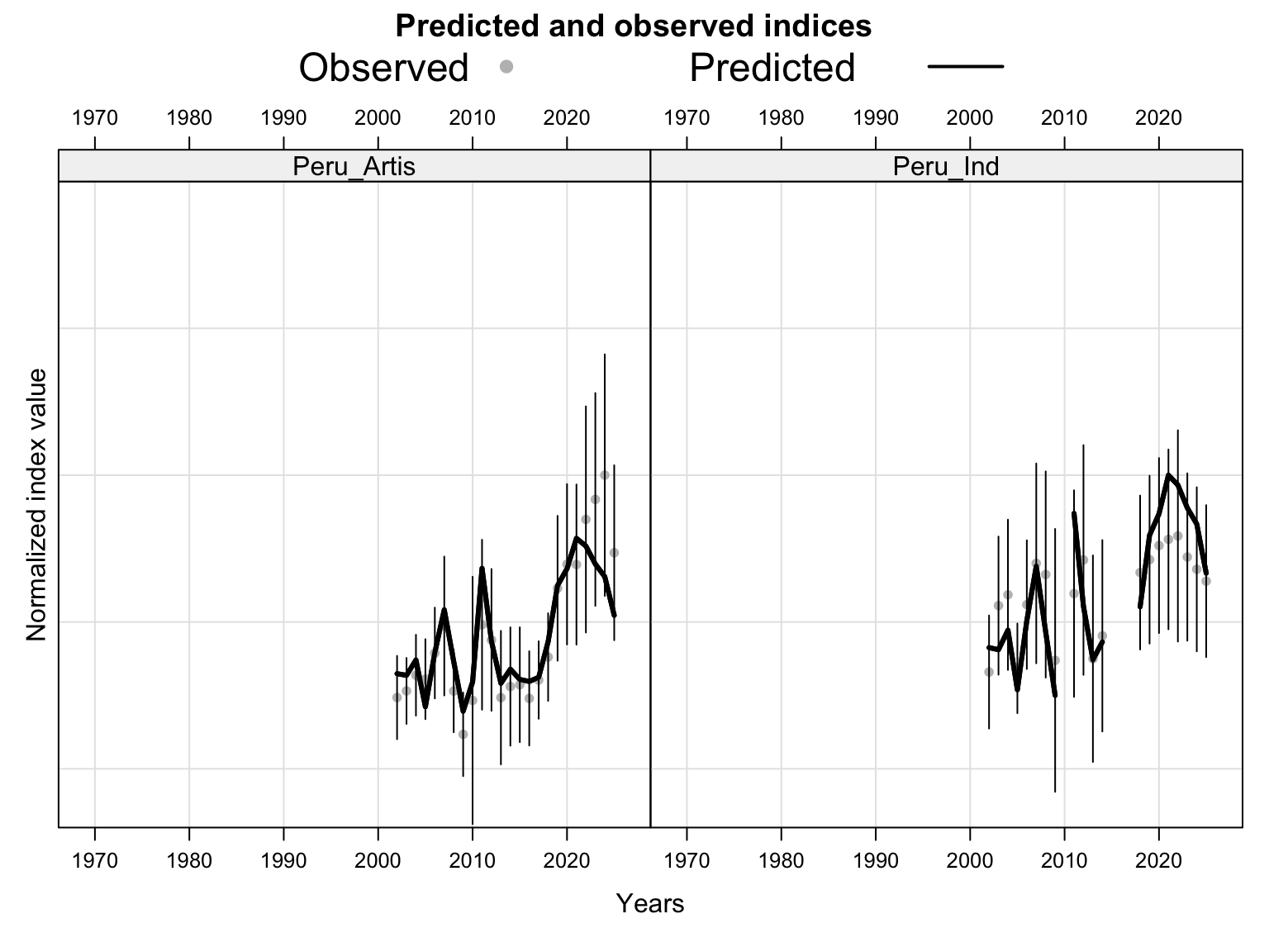
The post-benchmark model developments introduce new nominal Peruvian CPUE indices separated by fleet. The industrial and artisanal series both extend from 2002-2025. The CPUE values are calculated as total observed catch divided by the product of the total number of trips and mean vessel capacity. The industrial series includes a 1% annual effort-efficiency adjustment, whereas the artisanal series is left unadjusted from the observed effort data.
Both Peruvian CPUE series are assigned an average CV of 30%, compared with 20% for the other CPUE indices. Annual CVs vary with sampling coverage and are bounded below at a minimum CV of 20%. Years with no industrial CPUE observation retain the coverage-based CV but are not assigned an index value.
| Year | Industrial CPUE | With 1% creep | SD CPUE | CV | Sampling coverage |
|---|---|---|---|---|---|
| 2002 | 0.205486 | 0.205486 | 0.061259 | 0.298 | 30% |
| 2003 | 0.349850 | 0.346386 | 0.074805 | 0.216 | 58% |
| 2004 | 0.376780 | 0.369356 | 0.081379 | 0.220 | 56% |
| 2005 | 0.219693 | 0.213232 | 0.048549 | 0.228 | 52% |
| 2006 | 0.362611 | 0.348462 | 0.069692 | 0.200 | 73% |
| 2007 | 0.458303 | 0.436060 | 0.108192 | 0.248 | 44% |
| 2008 | 0.437844 | 0.412469 | 0.111641 | 0.271 | 37% |
| 2009 | 0.246792 | 0.230187 | 0.142322 | 0.618 | 7% |
| 2010 | NA | NA | NA | 0.922 | 3% |
| 2011 | 0.406734 | 0.371893 | 0.111876 | 0.301 | 30% |
| 2012 | 0.489588 | 0.443218 | 0.124367 | 0.281 | 34% |
| 2013 | 0.260740 | 0.233707 | 0.111849 | 0.479 | 12% |
| 2014 | 0.318137 | 0.282330 | 0.103625 | 0.367 | 20% |
| 2015 | NA | NA | NA | 0.349 | 22% |
| 2016 | NA | NA | NA | 0.341 | 23% |
| 2017 | NA | NA | NA | 0.223 | 55% |
| 2018 | 0.488574 | 0.416666 | 0.083333 | 0.200 | 71% |
| 2019 | 0.525740 | 0.443923 | 0.090851 | 0.205 | 65% |
| 2020 | 0.566820 | 0.473871 | 0.094774 | 0.200 | 68% |
| 2021 | 0.588301 | 0.486961 | 0.097392 | 0.200 | 69% |
| 2022 | 0.603181 | 0.494334 | 0.114390 | 0.231 | 50% |
| 2023 | 0.554019 | 0.449548 | 0.090618 | 0.202 | 67% |
| 2024 | 0.527146 | 0.423507 | 0.088856 | 0.210 | 61% |
| 2025 | 0.500858 | 0.398403 | 0.082289 | 0.207 | 63% |
| Year | Artisanal CPUE | SD CPUE | CV | Sampling coverage |
|---|---|---|---|---|
| 2002 | 0.163213 | 0.048657 | 0.298 | 30% |
| 2003 | 0.178359 | 0.038518 | 0.216 | 58% |
| 2004 | 0.214296 | 0.047215 | 0.220 | 56% |
| 2005 | 0.205230 | 0.046728 | 0.228 | 52% |
| 2006 | 0.265058 | 0.053012 | 0.200 | 73% |
| 2007 | 0.326913 | 0.081111 | 0.248 | 44% |
| 2008 | 0.178009 | 0.048181 | 0.271 | 37% |
| 2009 | 0.078910 | 0.048789 | 0.618 | 7% |
| 2010 | 0.156592 | 0.144364 | 0.922 | 3% |
| 2011 | 0.329883 | 0.099238 | 0.301 | 30% |
| 2012 | 0.295120 | 0.082811 | 0.281 | 34% |
| 2013 | 0.162969 | 0.077995 | 0.479 | 12% |
| 2014 | 0.188358 | 0.069134 | 0.367 | 20% |
| 2015 | 0.192454 | 0.067077 | 0.349 | 22% |
| 2016 | 0.161210 | 0.055045 | 0.341 | 23% |
| 2017 | 0.203272 | 0.045238 | 0.223 | 55% |
| 2018 | 0.255798 | 0.051160 | 0.200 | 71% |
| 2019 | 0.413299 | 0.084584 | 0.205 | 65% |
| 2020 | 0.468169 | 0.093634 | 0.200 | 68% |
| 2021 | 0.467559 | 0.093512 | 0.200 | 69% |
| 2022 | 0.570841 | 0.132094 | 0.231 | 50% |
| 2023 | 0.616602 | 0.124292 | 0.202 | 67% |
| 2024 | 0.672200 | 0.141035 | 0.210 | 61% |
| 2025 | 0.494612 | 0.102160 | 0.207 | 63% |
model_descriptions |>
  filter(model %in% core_versions) |>
  select(model_label, role, description) |>
  knitr::kable(
    col.names = c("Model", "Role", "Description"),
    align = "lll"
  ) |>
kableExtra::kable_styling(full_width = FALSE)| Model | Role | Description |
|---|---|---|
| 0.00 | SCW16 baseline | SCW16 baseline configuration retained to anchor the model-development bridge. |
| 0.14 | SCW16 final bridge | SCW16 proposed final configuration used as the main comparison point for subsequent development. |
| 0.15 | Model development | Uses the 0.15 data treatment, including separate nominal Peruvian artisanal and industrial CPUE indices. The Peruvian CPUE q random walks are removed. |
| 0.16 | Productivity-regime development | Same data treatment as 0.15. For h2, the change is in productivity-regime specifications: stock 2 is represented with one productivity regime rather than separate pre/post regimes. The h1_0.15.ctl and h1_0.16.ctl files have the same biological and data specifications. |
The source controls are read from /Users/jim/_mymods/sprfmo/jjm/assessment/config. The rendered document can be run from the SCW17 repository or from the JJM assessment checkout; set JJM_ASSESSMENT_DIR if the assessment directory is not found automatically.
control_inventory |>
  filter(model %in% core_versions) |>
  transmute(
    Hypothesis = hypothesis,
    Model = model_label,
    `Control file` = control_file,
    `Data file` = data_file,
    `Model name` = model_name,
    `Stocks` = nstocks,
    `Productivity regimes by stock` = nregby_stock,
    `Recruitment matrix` = rec_matrix,
    `SR years` = nyrs_sr,
    `Number of q terms` = n_q,
    `Has model output` = completed_output
  ) |>
  knitr::kable(align = c(rep("l", 9), "r", "l")) |>
kableExtra::kable_styling(full_width = FALSE, font_size = 12)| Hypothesis | Model | Control file | Data file | Model name | Stocks | Productivity regimes by stock | Recruitment matrix | SR years | Number of q terms | Has model output |
|---|---|---|---|---|---|---|---|---|---|---|
| h1 | 0.00 | h1_0.00.ctl | 0.00.dat | h1_0.00 | 1 | 1 | 1 | 23 | 7 | TRUE |
| h2 | 0.00 | h2_0.00.ctl | 0.00.dat | h2_0.00 | 2 | 1 2 | 1 2 3 | 23 27 16 | 7 | TRUE |
| h1 | 0.14 | h1_0.14.ctl | 0.14.dat | h1_0.14 | 1 | 1 | 1 | 23 | 5 | TRUE |
| h2 | 0.14 | h2_0.14.ctl | 0.14.dat | h2_0.14 | 2 | 1 2 | 1 2 3 | 23 27 16 | 5 | TRUE |
| h1 | 0.15 | h1_0.15.ctl | 0.15.dat | h1_0.15 | 1 | 1 | 1 | 23 | 6 | TRUE |
| h2 | 0.15 | h2_0.15.ctl | 0.15.dat | h2_0.15 | 2 | 1 2 | 1 2 3 | 23 27 16 | 6 | TRUE |
| h1 | 0.16 | h1_0.16.ctl | 0.15.dat | h1_0.16 | 1 | 1 | 1 | 23 | 6 | TRUE |
| h2 | 0.16 | h2_0.16.ctl | 0.15.dat | h2_0.16 | 2 | 1 1 | 1 2 | 23 47 | 6 | TRUE |
The 0.00 configuration is retained as the SCW16 baseline bridge run. The 0.14 configuration is retained as the SCW16 proposed final model. Model 0.15 starts from the 0.14 line of development and changes the Peruvian CPUE treatment to use separate nominal artisanal and industrial CPUE indices. The Peruvian CPUE catchability random walks used in 0.14 are not estimated for those two nominal indices in 0.15.
Model 0.16 uses the same data treatment as 0.15 but changes the productivity-regime specification. Under the two-stock hypothesis, h2_0.15.ctl retains the separate stock-2 productivity regimes and the associated regime shift used in the SCW16 model line, whereas h2_0.16.ctl combines stock 2 into one productivity regime. Under the single-stock hypothesis, h1_0.15.ctl and h1_0.16.ctl have the same biological and data specifications; the model-development distinction is therefore only meaningful for the two-stock productivity-regime specification.
fit_summary |>
  filter(model %in% core_versions) |>
  mutate(
    nll = round(nll, 3),
    max_gradient = signif(max_gradient, 4)
  ) |>
  select(hypothesis, model_label, model_id, nopar, nll, max_gradient) |>
  knitr::kable(
    col.names = c("Hypothesis", "Model", "Run", "N parameters", "NLL", "Max gradient"),
    align = "lllrrr"
  ) |>
kableExtra::kable_styling(full_width = FALSE)| Hypothesis | Model | Run | N parameters | NLL | Max gradient |
|---|---|---|---|---|---|
| h1 | 0.00 | h1_0.00 | 1865 | 1371.555 | 0.0001980 |
| h2 | 0.00 | h2_0.00 | 1648 | 1197.202 | 0.0002031 |
| h1 | 0.14 | h1_0.14 | 1844 | 1301.527 | 0.0002059 |
| h2 | 0.14 | h2_0.14 | 1935 | 1196.391 | 0.0002301 |
| h1 | 0.15 | h1_0.15 | 1829 | 1370.909 | 0.0003086 |
| h2 | 0.15 | h2_0.15 | 1905 | 1226.735 | 0.0002159 |
| h1 | 0.16 | h1_0.16 | 1552 | 1372.316 | 0.0001519 |
| h2 | 0.16 | h2_0.16 | 1626 | 1197.156 | 0.0003552 |
if (nrow(terminal_metrics)) {
  terminal_metrics |>
    mutate(
      ssb = round(ssb),
      total_biomass = round(total_biomass),
      recruitment = round(recruitment),
      max_total_f_at_age = round(max_total_f_at_age, 3)
    ) |>
    select(hypothesis, model_label, stock, year, ssb, total_biomass, recruitment, max_total_f_at_age) |>
    knitr::kable(
      col.names = c("Hypothesis", "Model", "Stock", "Year", "SSB", "Total biomass", "Recruitment", "Max total F at age"),
      align = "llllrrrr"
    ) |>
    kableExtra::kable_styling(full_width = FALSE)
} else {
  knitr::kable(tibble(note = "No model outputs were available."))
}| Hypothesis | Model | Stock | Year | SSB | Total biomass | Recruitment | Max total F at age |
|---|---|---|---|---|---|---|---|
| h1 | 0.00 | Stock_1 | 2025 | 16003 | 22908 | 17657 | 0.516 |
| h2 | 0.00 | Stock_1 | 2025 | 10474 | 15630 | 15028 | 0.684 |
| h2 | 0.00 | Stock_2 | 2025 | 1095 | 1726 | 1176 | 0.494 |
| h1 | 0.14 | Stock_1 | 2025 | 5772 | 9678 | 12357 | 2.166 |
| h2 | 0.14 | Stock_1 | 2025 | 5398 | 9023 | 11709 | 1.812 |
| h2 | 0.14 | Stock_2 | 2025 | 303 | 698 | 998 | 1.949 |
| h1 | 0.15 | Stock_1 | 2025 | 6897 | 11134 | 12941 | 2.768 |
| h2 | 0.15 | Stock_1 | 2025 | 5398 | 9024 | 11710 | 1.820 |
| h2 | 0.15 | Stock_2 | 2025 | 331 | 733 | 1006 | 1.233 |
| h1 | 0.16 | Stock_1 | 2025 | 6834 | 11082 | 13208 | 2.745 |
| h2 | 0.16 | Stock_1 | 2025 | 8050 | 12528 | 13935 | 2.525 |
| h2 | 0.16 | Stock_2 | 2025 | 4194 | 5956 | 3086 | 0.144 |
if (nrow(terminal_deltas)) {
  terminal_deltas |>
    mutate(across(ends_with("_delta_pct"), ~round(.x, 1))) |>
    select(hypothesis, model_label, stock, year, ends_with("_delta_pct")) |>
    knitr::kable(
      col.names = c("Hypothesis", "Model", "Stock", "Year", "SSB (%)", "Total biomass (%)", "Recruitment (%)", "Max total F at age (%)"),
      align = "llllrrrr"
    ) |>
    kableExtra::kable_styling(full_width = FALSE)
} else {
  knitr::kable(tibble(note = "Percent differences will populate after at least one comparison model and 0.14 have model output."))
}| Hypothesis | Model | Stock | Year | SSB (%) | Total biomass (%) | Recruitment (%) | Max total F at age (%) |
|---|---|---|---|---|---|---|---|
| h1 | 0.00 | Stock_1 | 2025 | 177.2 | 136.7 | 42.9 | -76.2 |
| h2 | 0.00 | Stock_1 | 2025 | 94.0 | 73.2 | 28.3 | -62.3 |
| h2 | 0.00 | Stock_2 | 2025 | 261.3 | 147.5 | 17.9 | -74.7 |
| h1 | 0.14 | Stock_1 | 2025 | 0.0 | 0.0 | 0.0 | 0.0 |
| h2 | 0.14 | Stock_1 | 2025 | 0.0 | 0.0 | 0.0 | 0.0 |
| h2 | 0.14 | Stock_2 | 2025 | 0.0 | 0.0 | 0.0 | 0.0 |
| h1 | 0.15 | Stock_1 | 2025 | 19.5 | 15.1 | 4.7 | 27.8 |
| h2 | 0.15 | Stock_1 | 2025 | 0.0 | 0.0 | 0.0 | 0.5 |
| h2 | 0.15 | Stock_2 | 2025 | 9.3 | 5.0 | 0.8 | -36.7 |
| h1 | 0.16 | Stock_1 | 2025 | 18.4 | 14.5 | 6.9 | 26.7 |
| h2 | 0.16 | Stock_1 | 2025 | 49.1 | 38.8 | 19.0 | 39.4 |
| h2 | 0.16 | Stock_2 | 2025 | 1284.1 | 753.8 | 209.4 | -92.6 |
The plots below compare the SC13 baseline (0.00), the SCW16 proposed final model (0.14), and the subsequent 0.15 and 0.16 model-development outputs. This section highlights issues identified after the benchmark workshop (SCW16) with the model configuration and the need to consider an alternative proposal for use in MSE operating-model conditioning. The comparisons are included here so that the subsequent 0.15 and 0.16 outputs can be interpreted relative to the SCW16 work.
h1_bridge <- NULL
h2_bridge <- NULL

if (length(bridge_plot_versions) >= 2) {
  h1_bridge <- safe_compare_models(paste0("h1_", bridge_plot_versions))
  h2_bridge <- safe_compare_models(paste0("h2_", bridge_plot_versions))
}plot_model_timeseries(paste0("h1_", comparison_plot_versions), "biomass", "Biomass")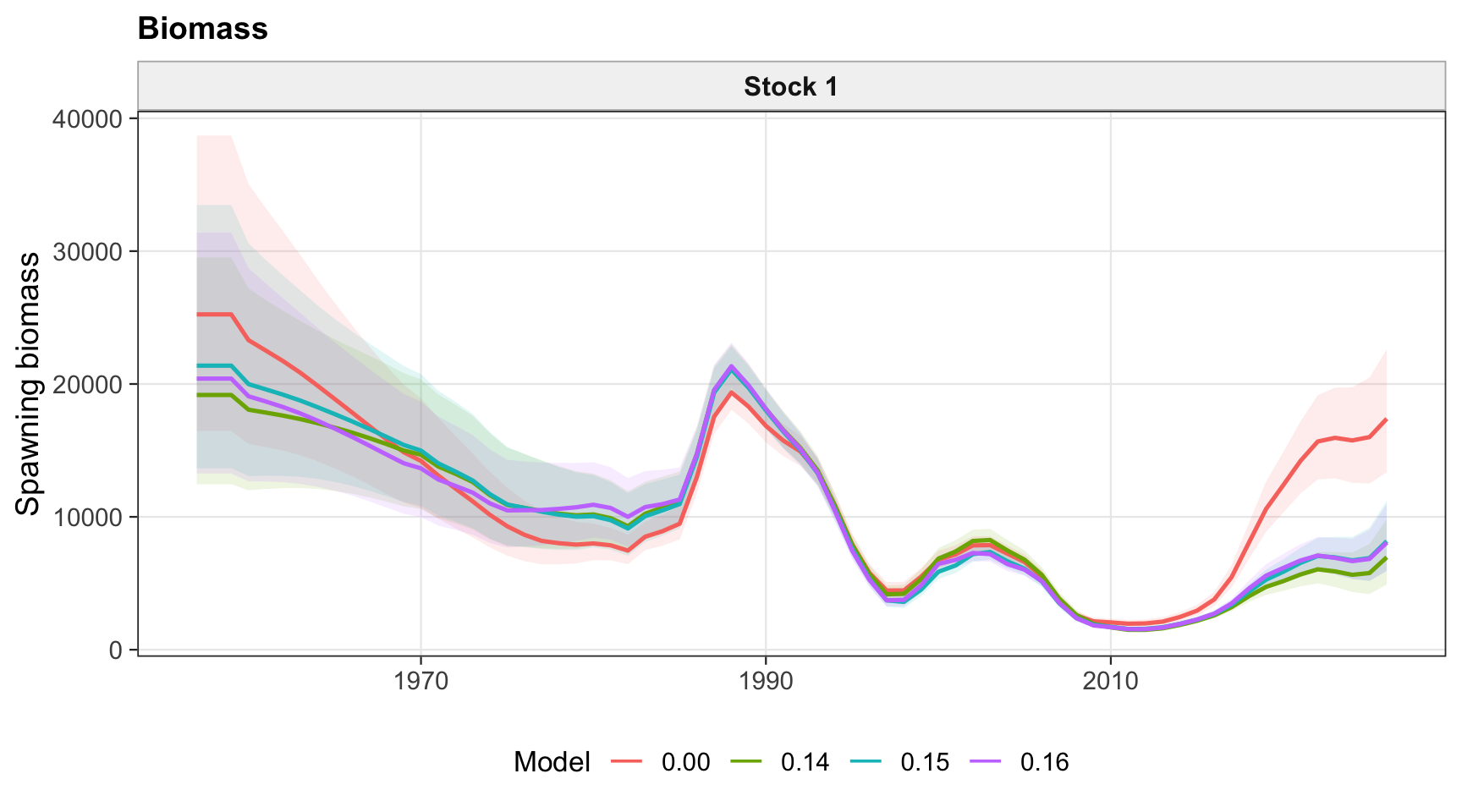
plot_model_timeseries(paste0("h1_", comparison_plot_versions), "recruitment", "Recruitment")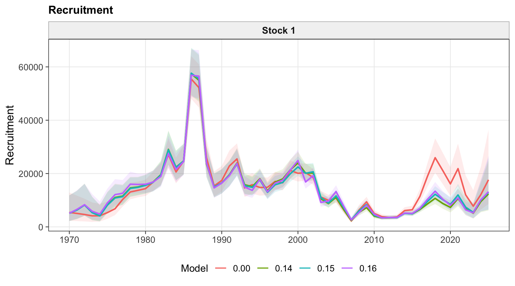
plot_model_timeseries(paste0("h1_", comparison_plot_versions), "ftot", "Total Fishing Mortality")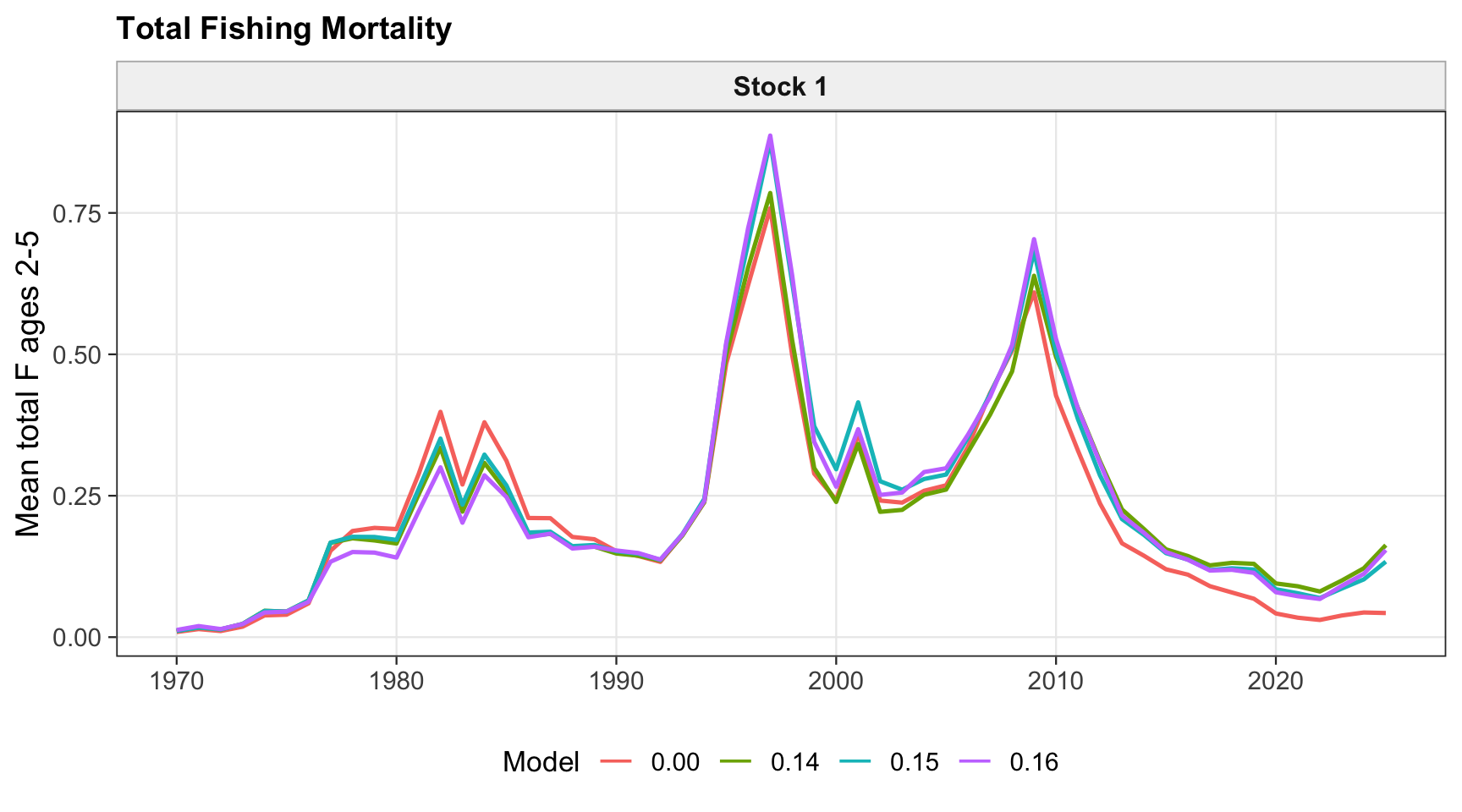
plot_model_timeseries(paste0("h2_", comparison_plot_versions), "biomass", "Biomass")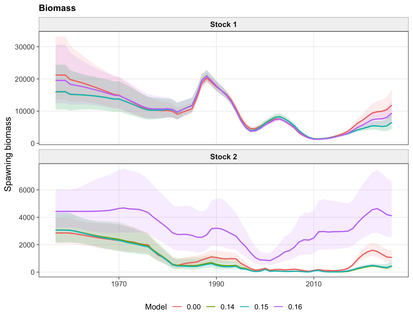
plot_model_timeseries(paste0("h2_", comparison_plot_versions), "recruitment", "Recruitment")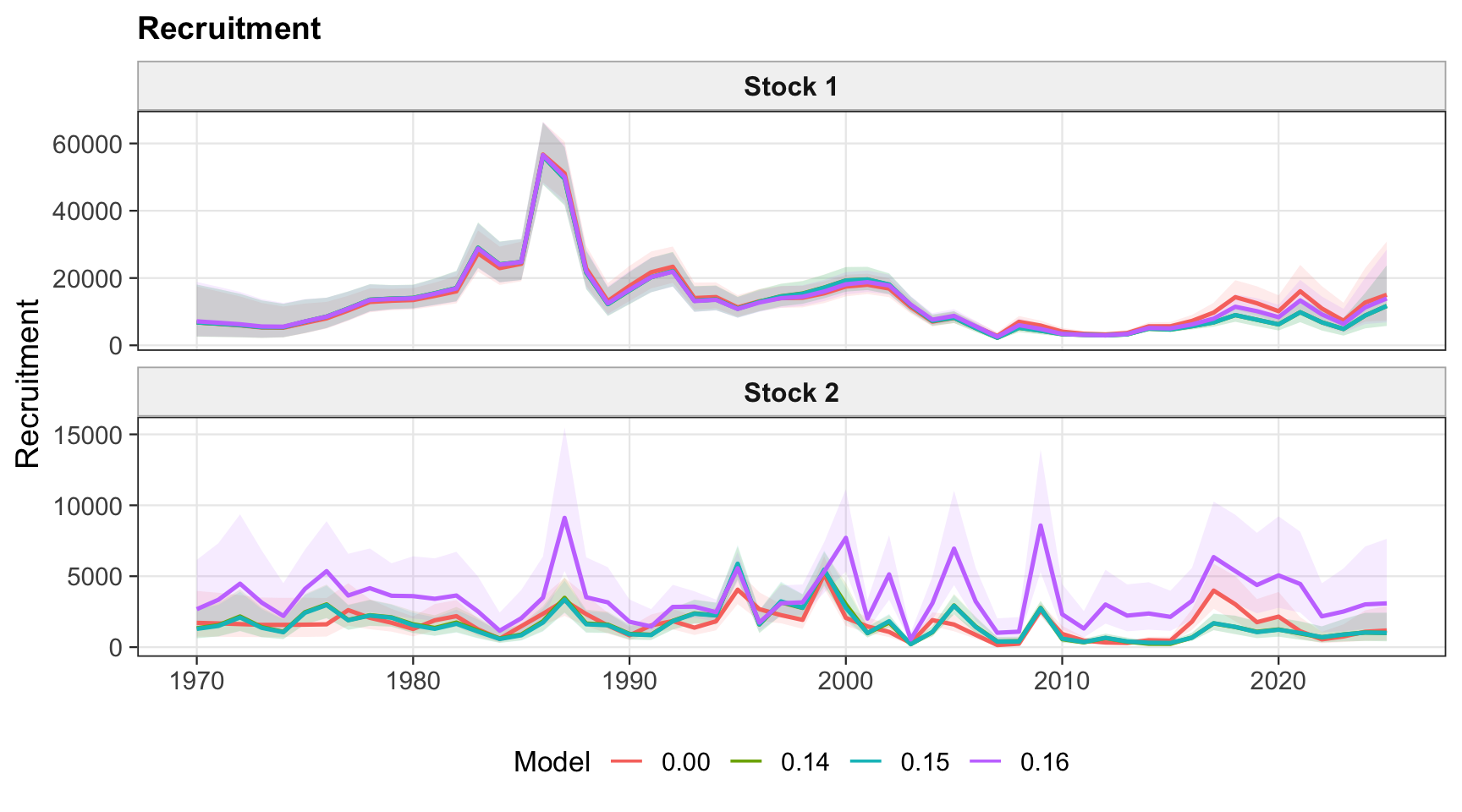
plot_model_timeseries(paste0("h2_", comparison_plot_versions), "ftot", "Total Fishing Mortality")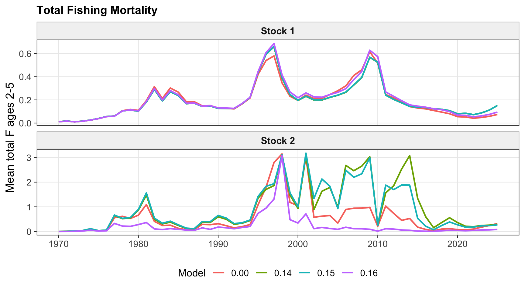
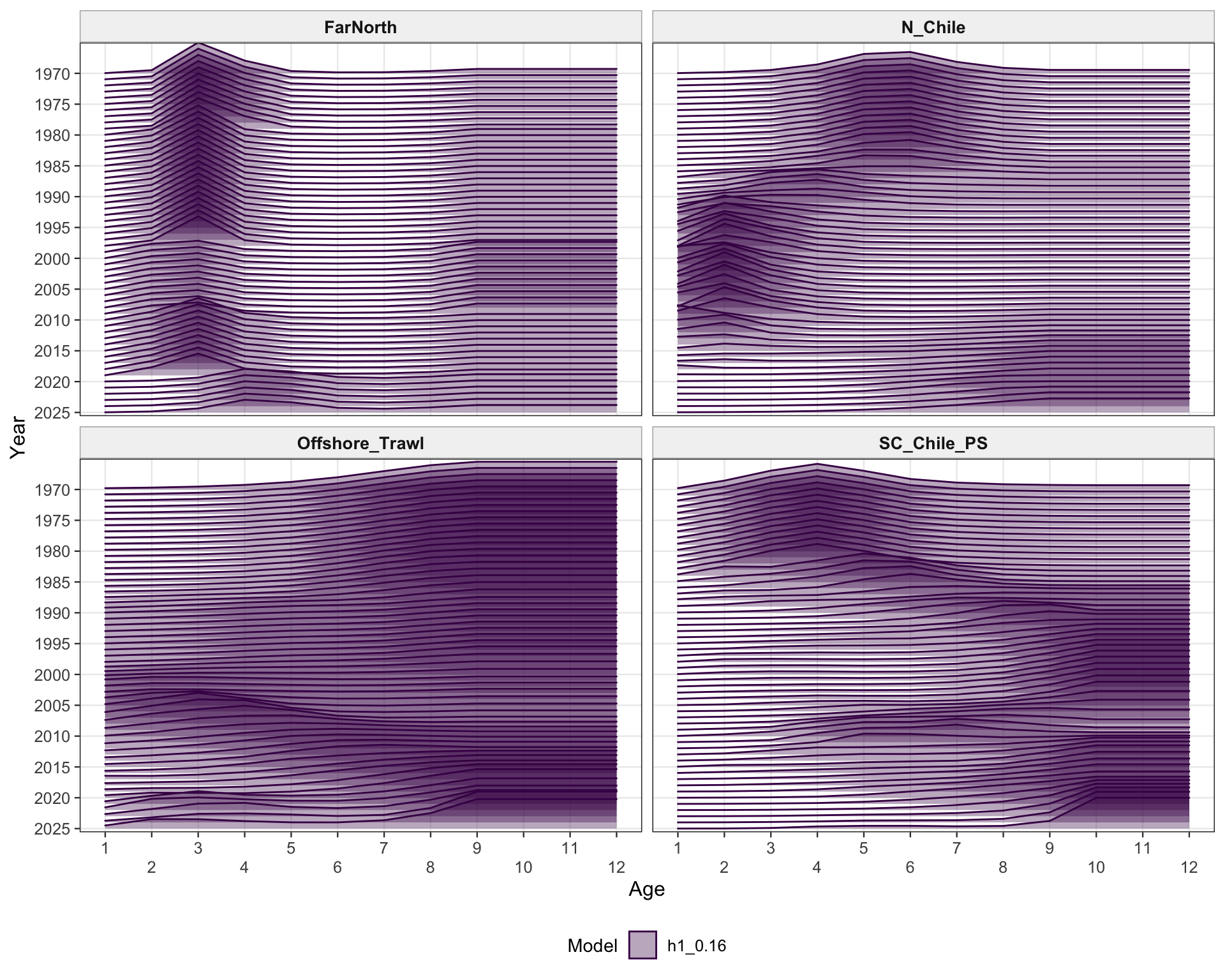
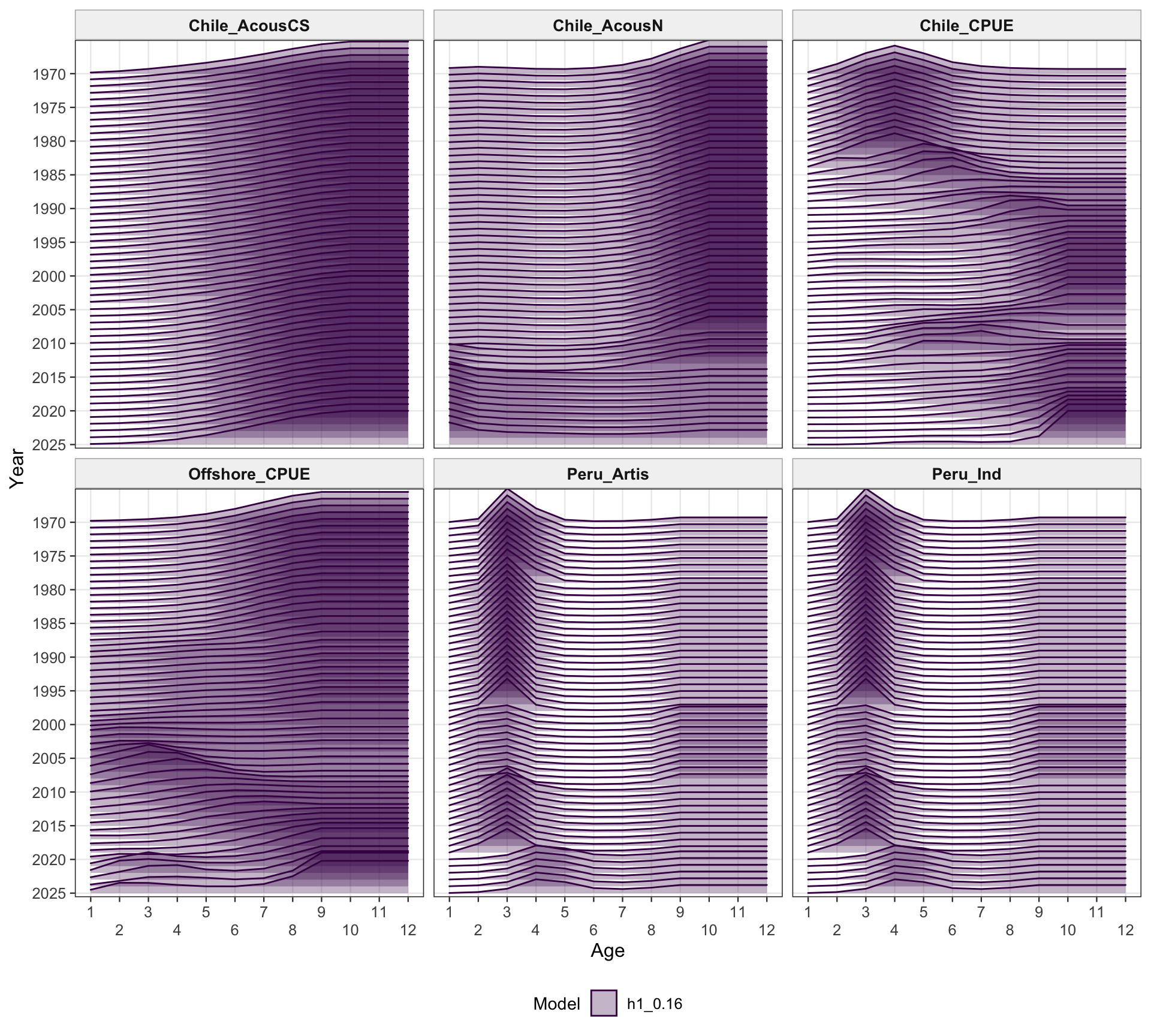
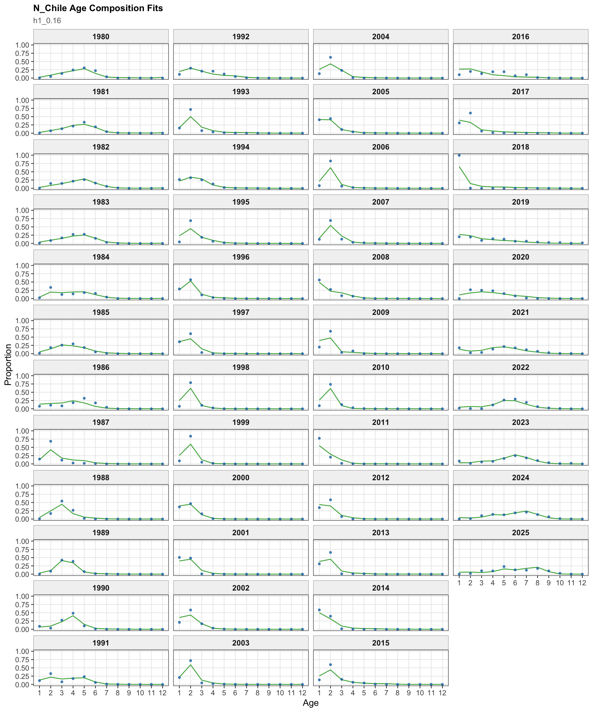
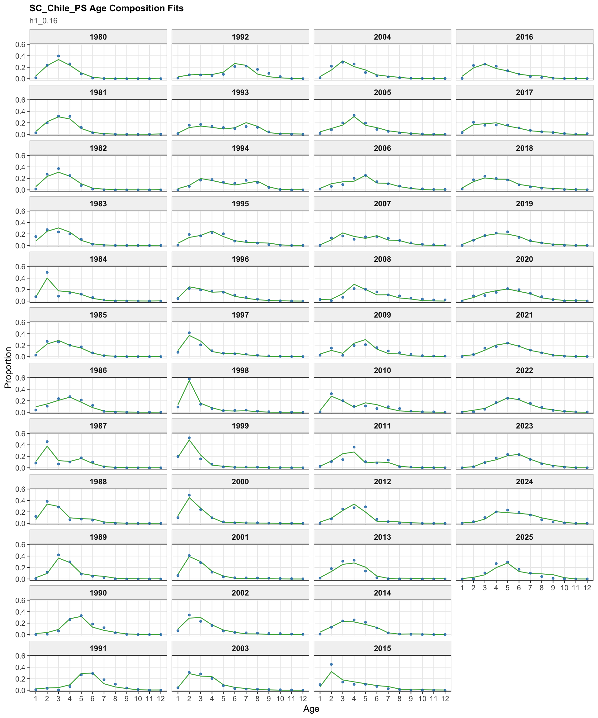
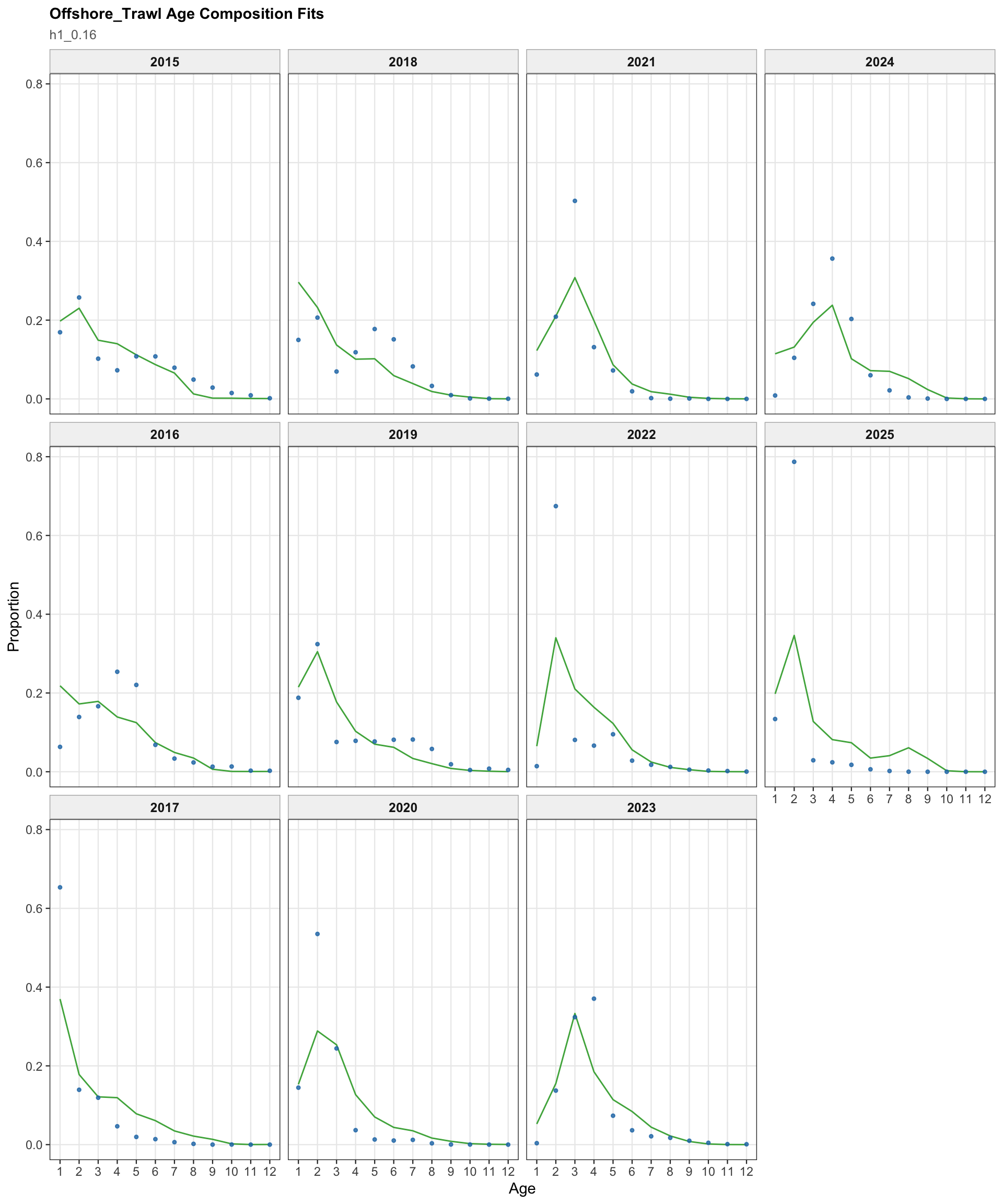
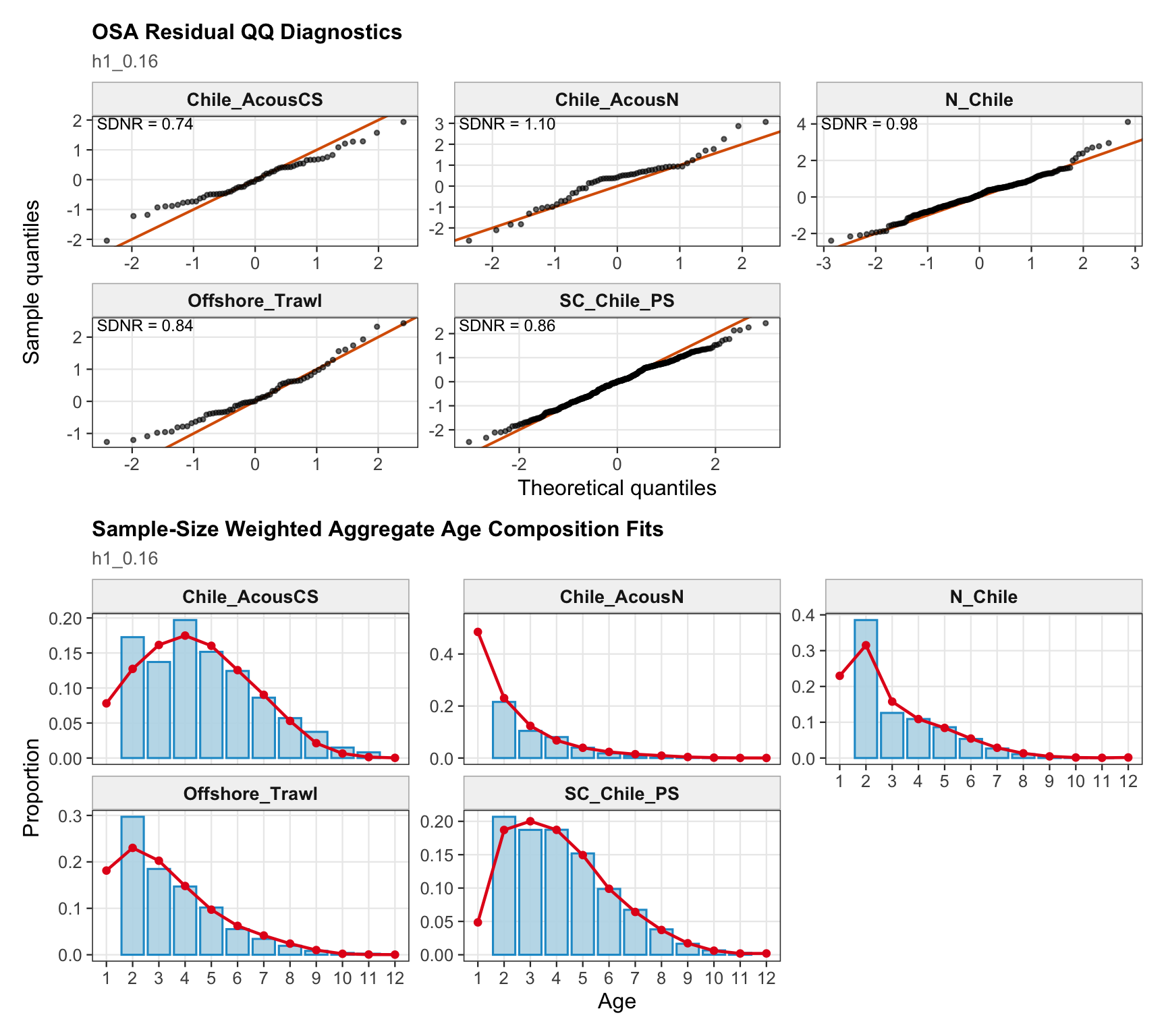
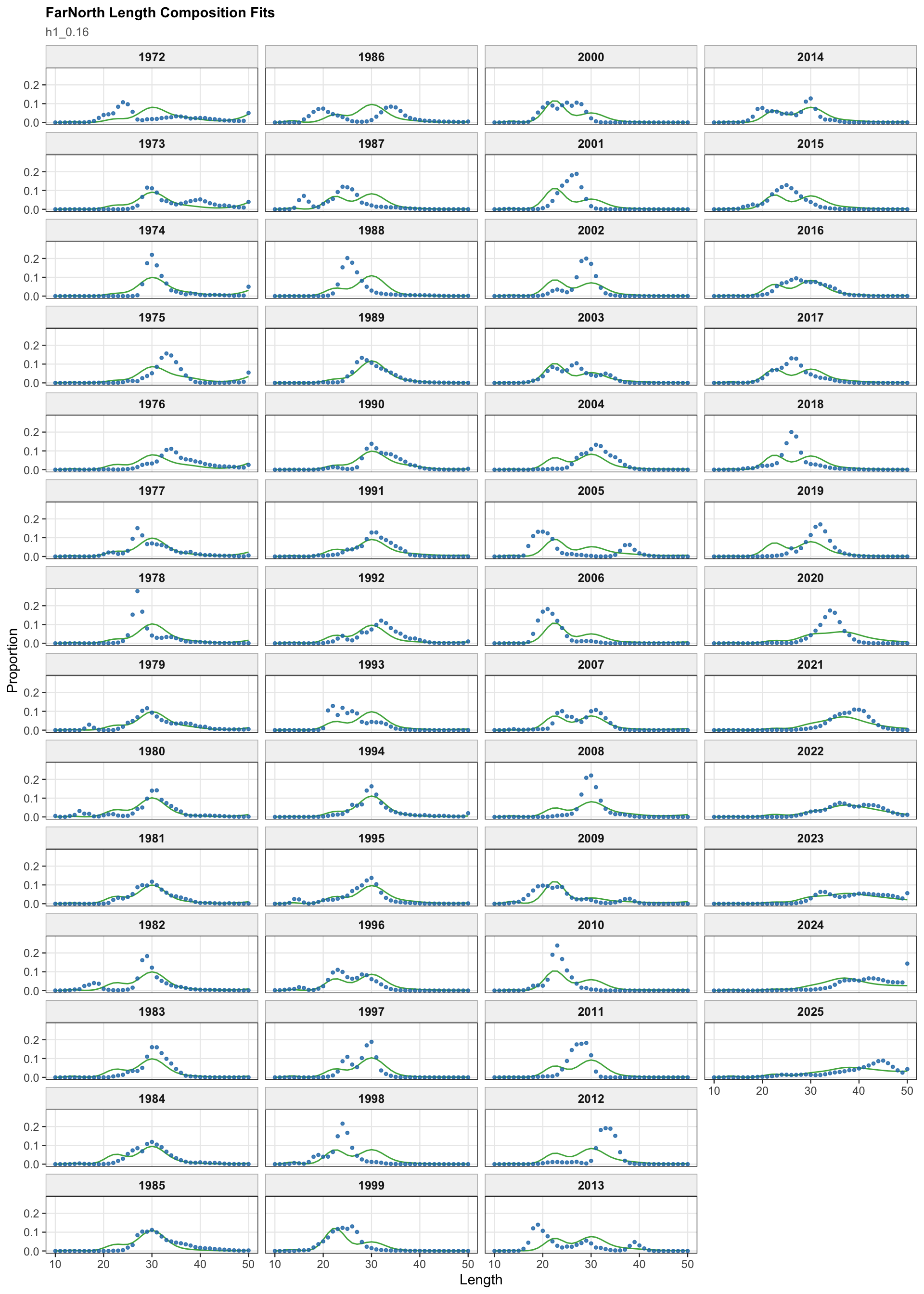
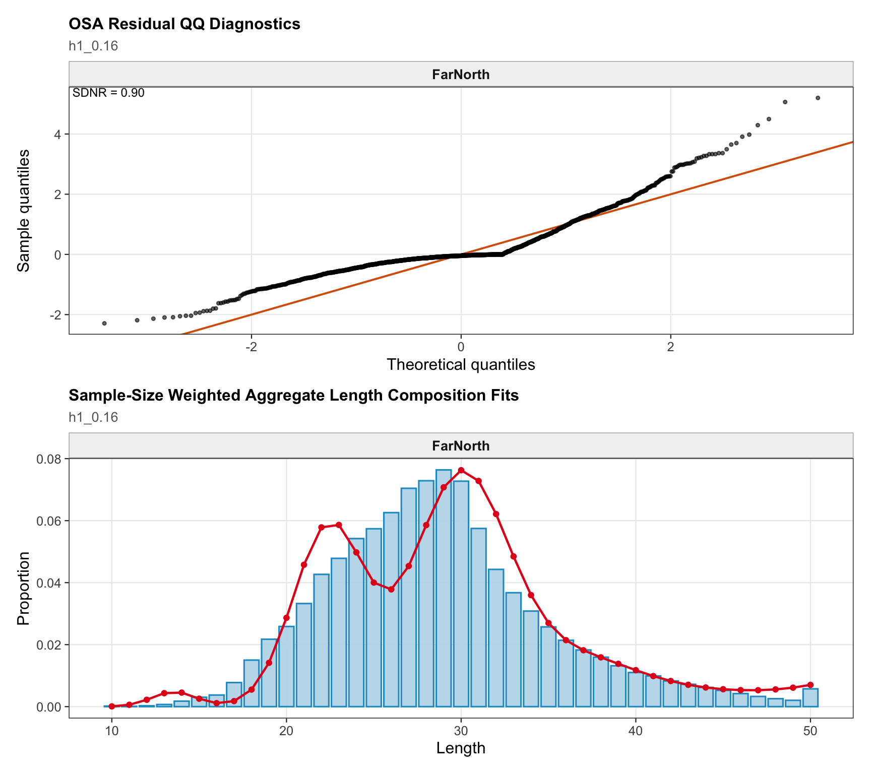
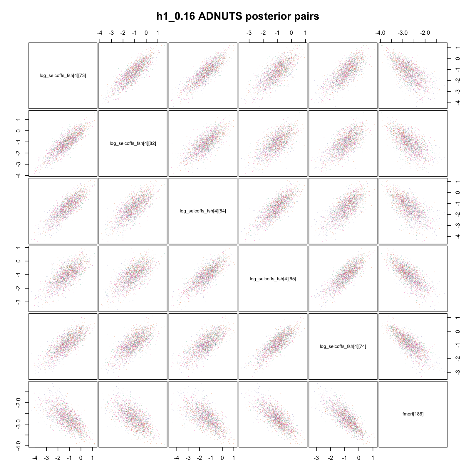
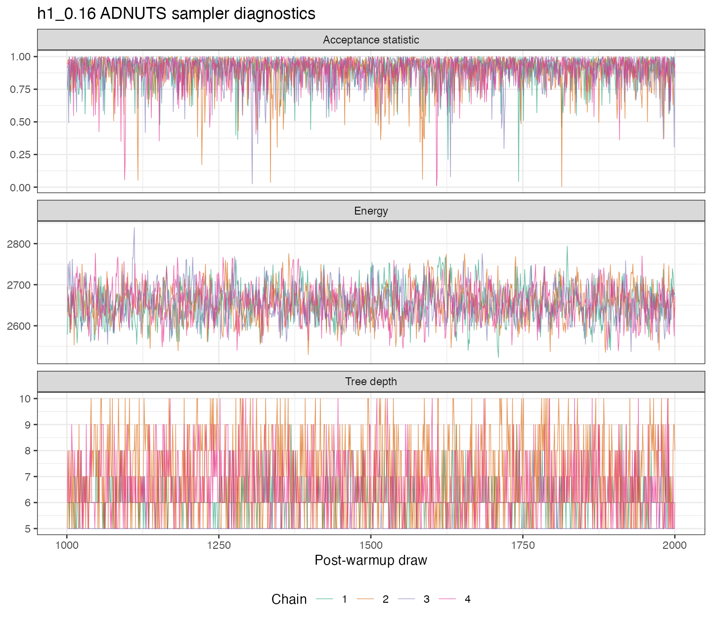
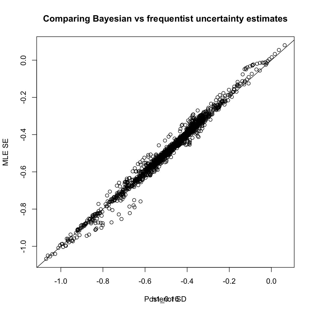
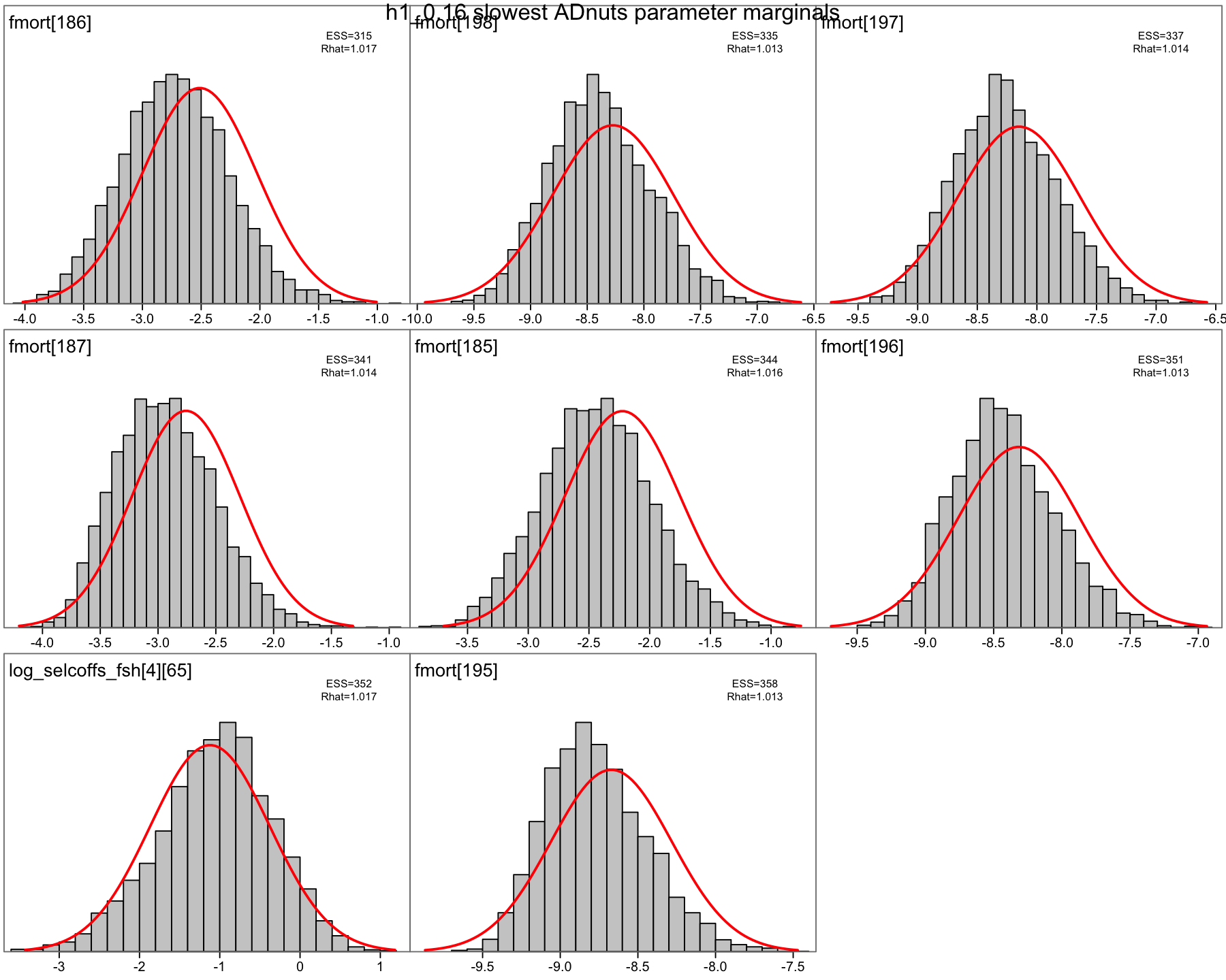
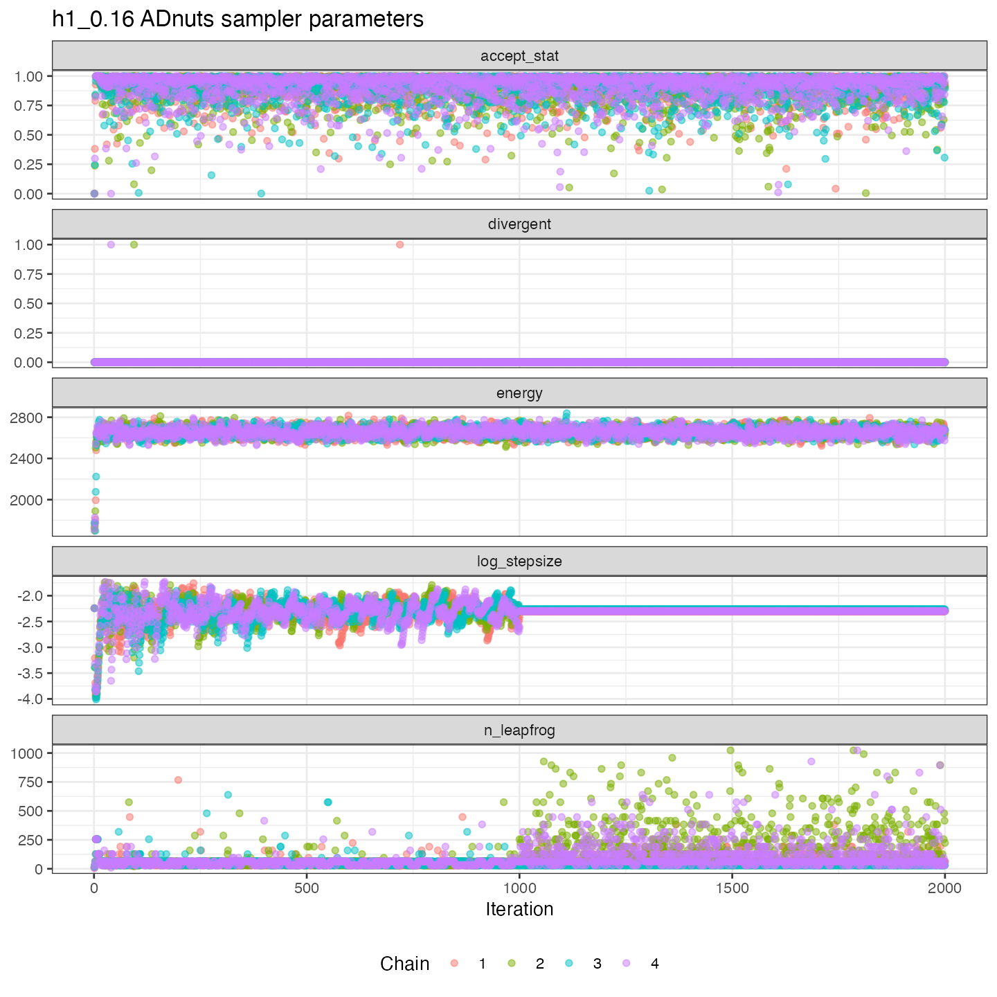
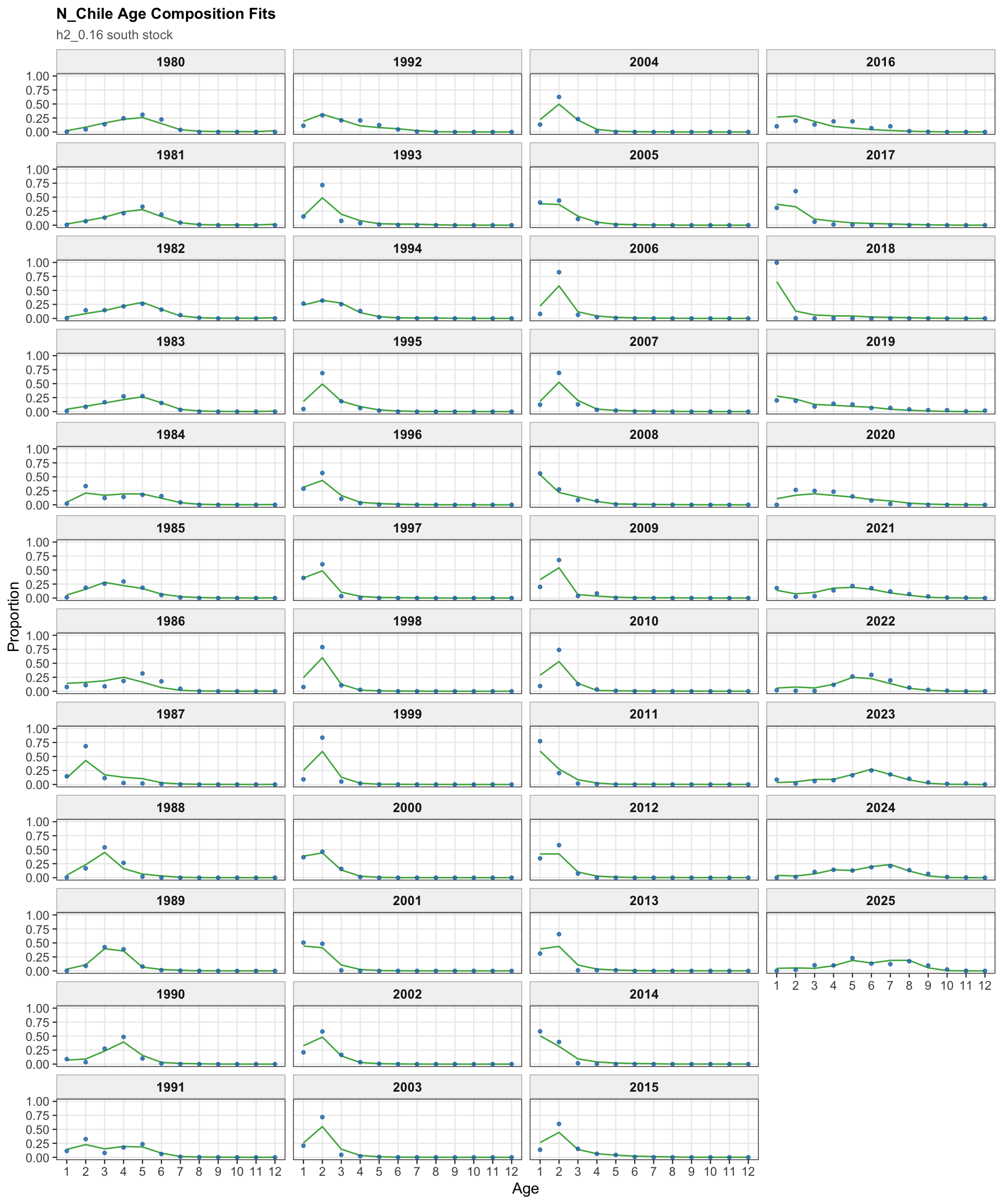
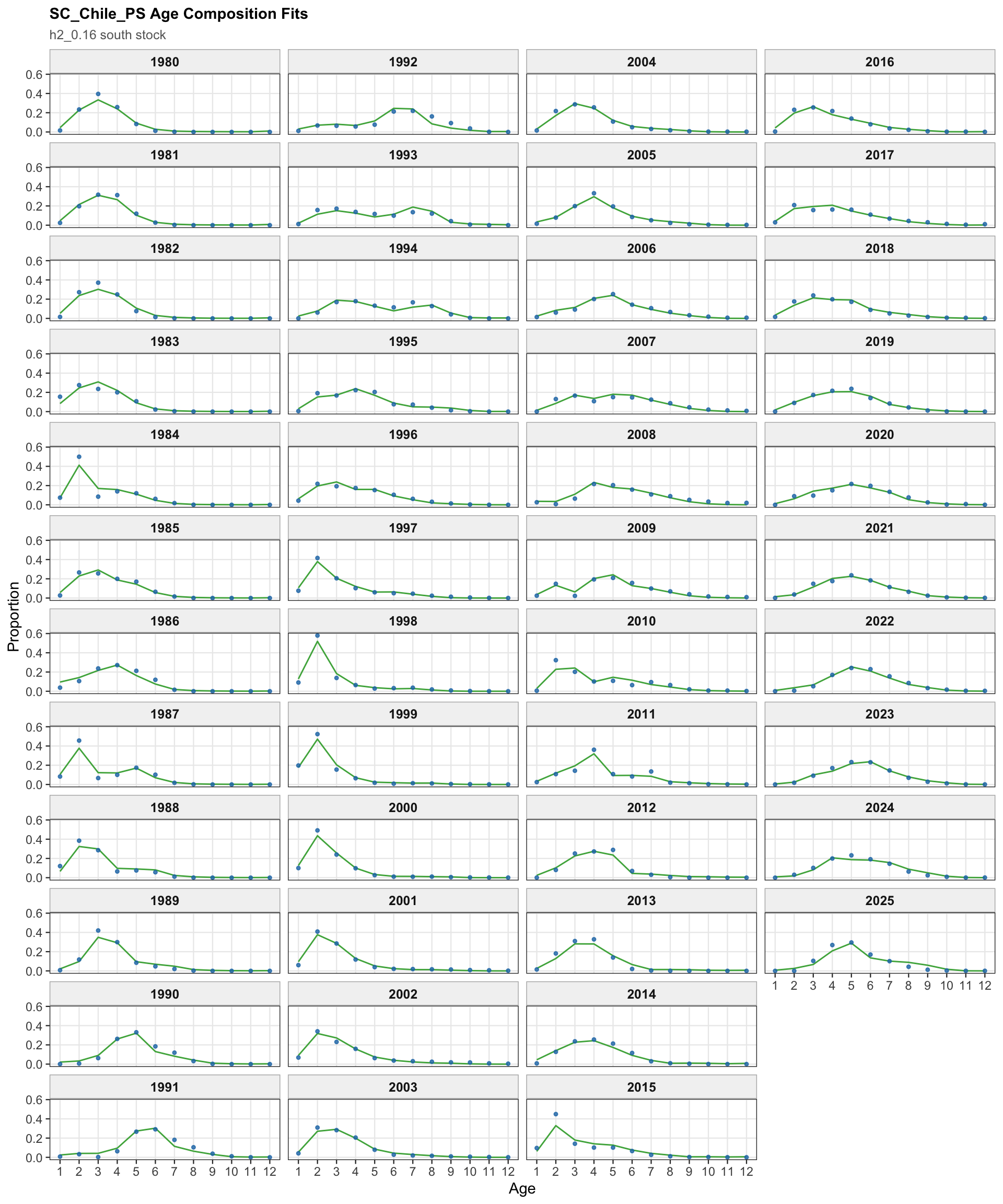
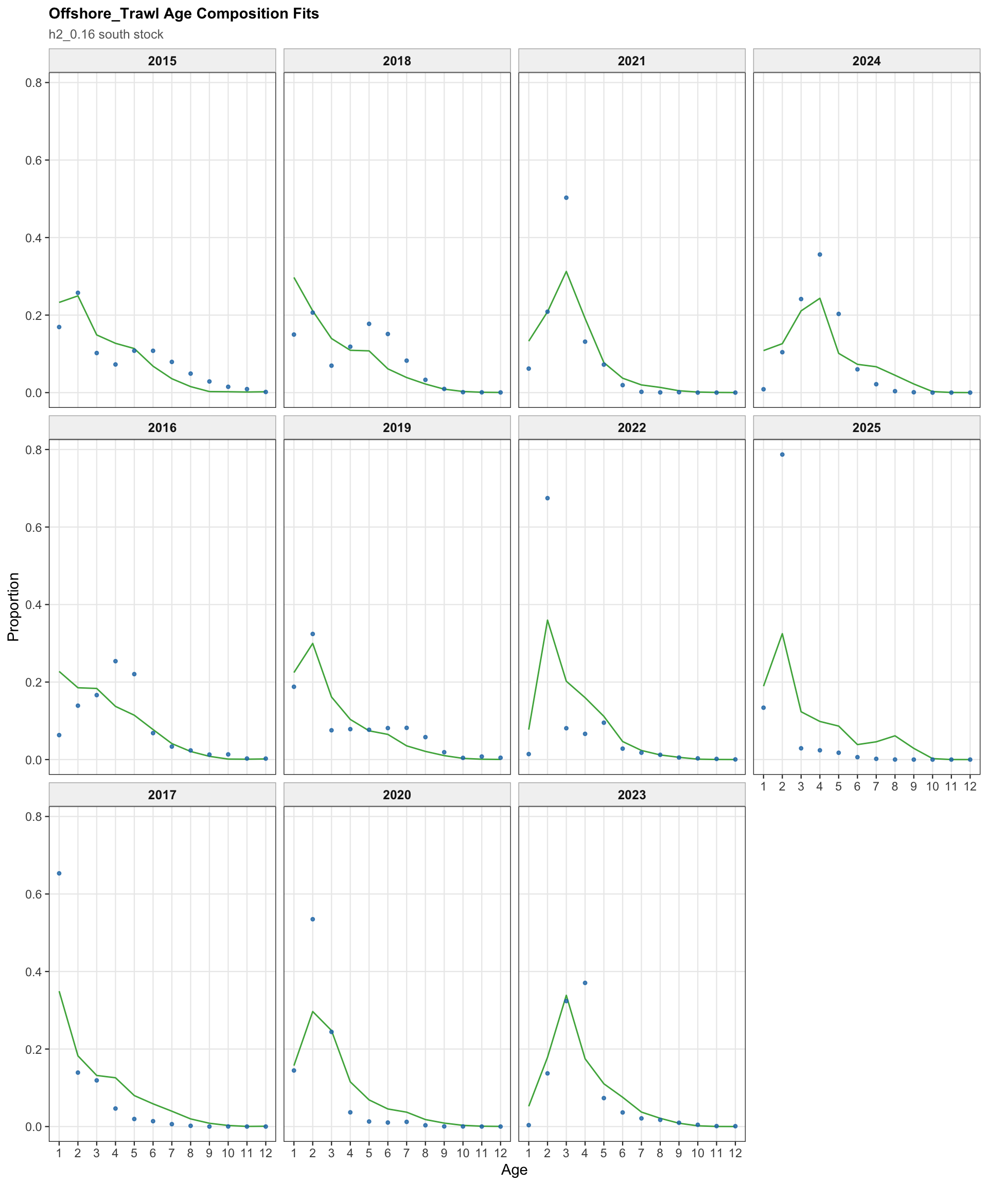
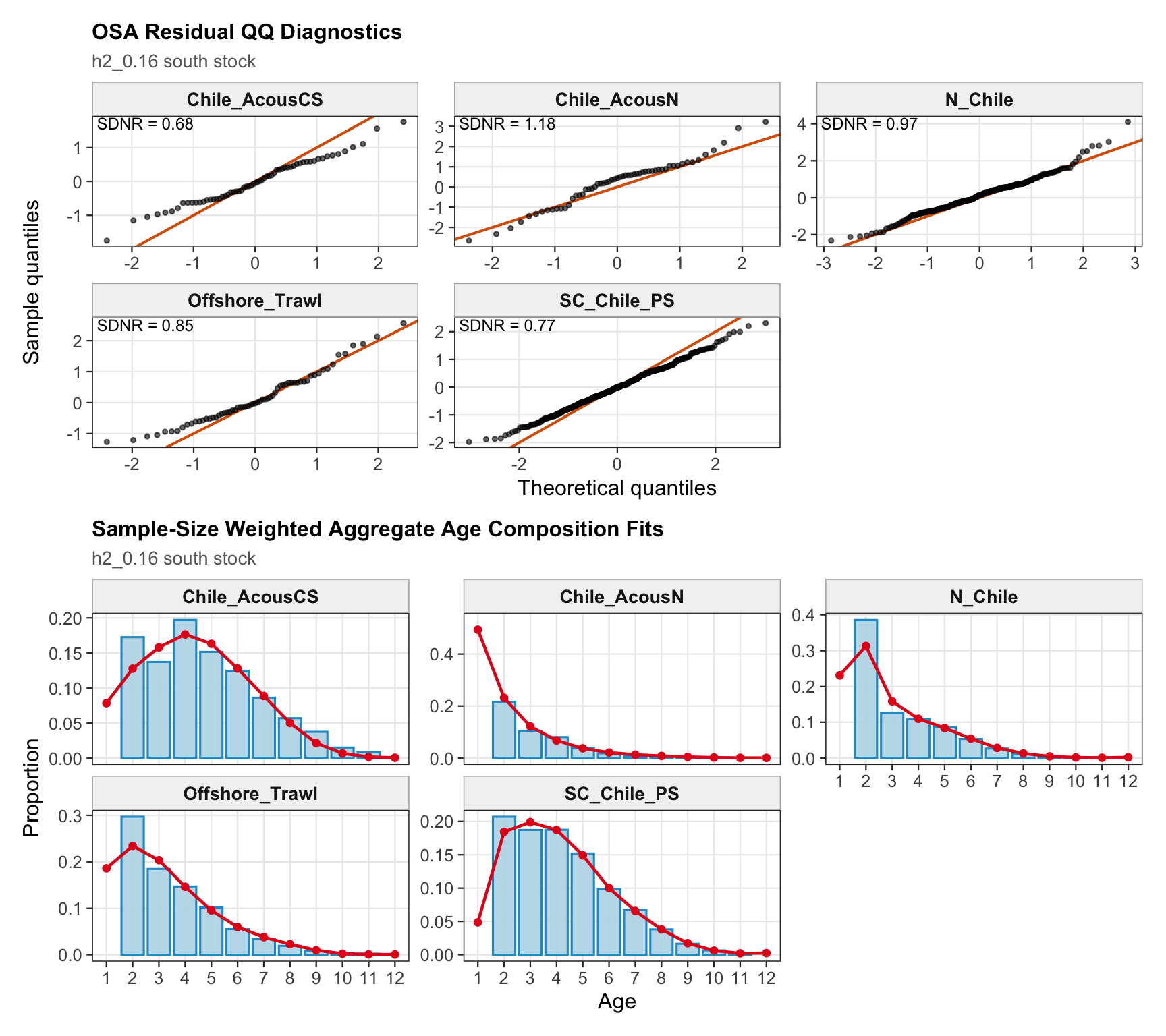
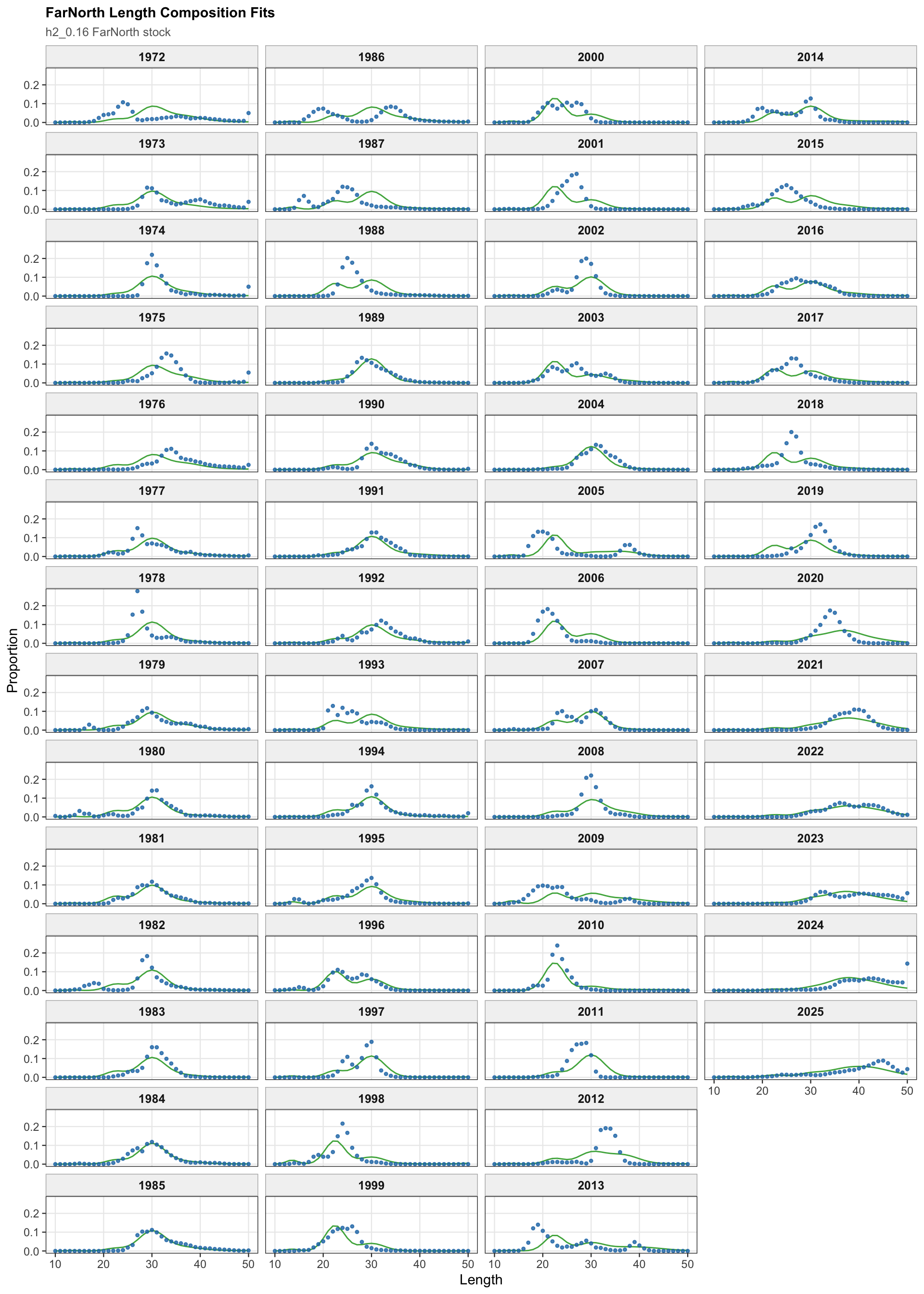
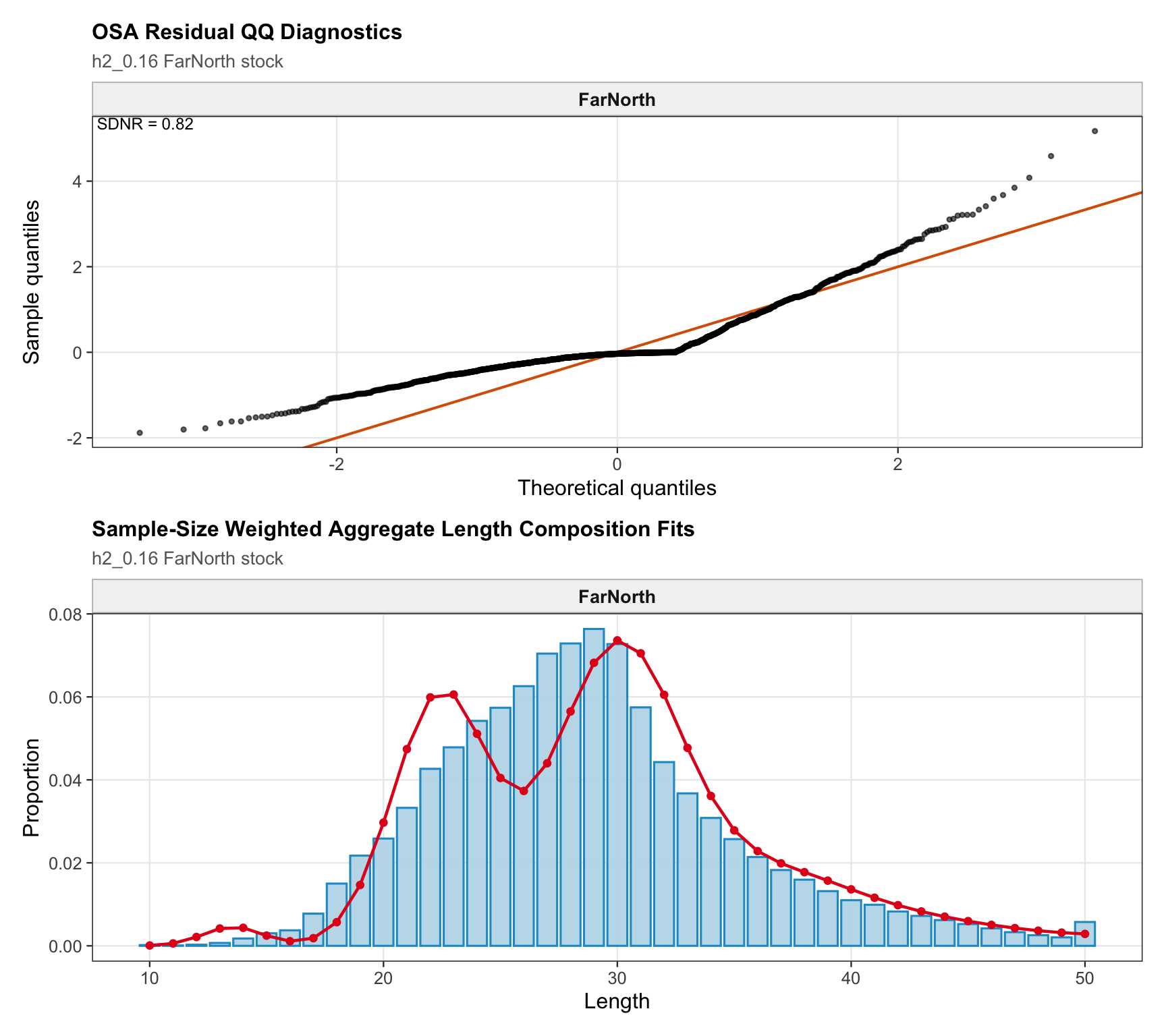
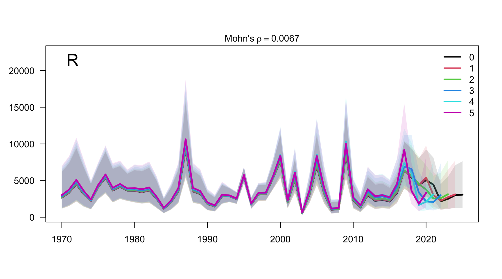
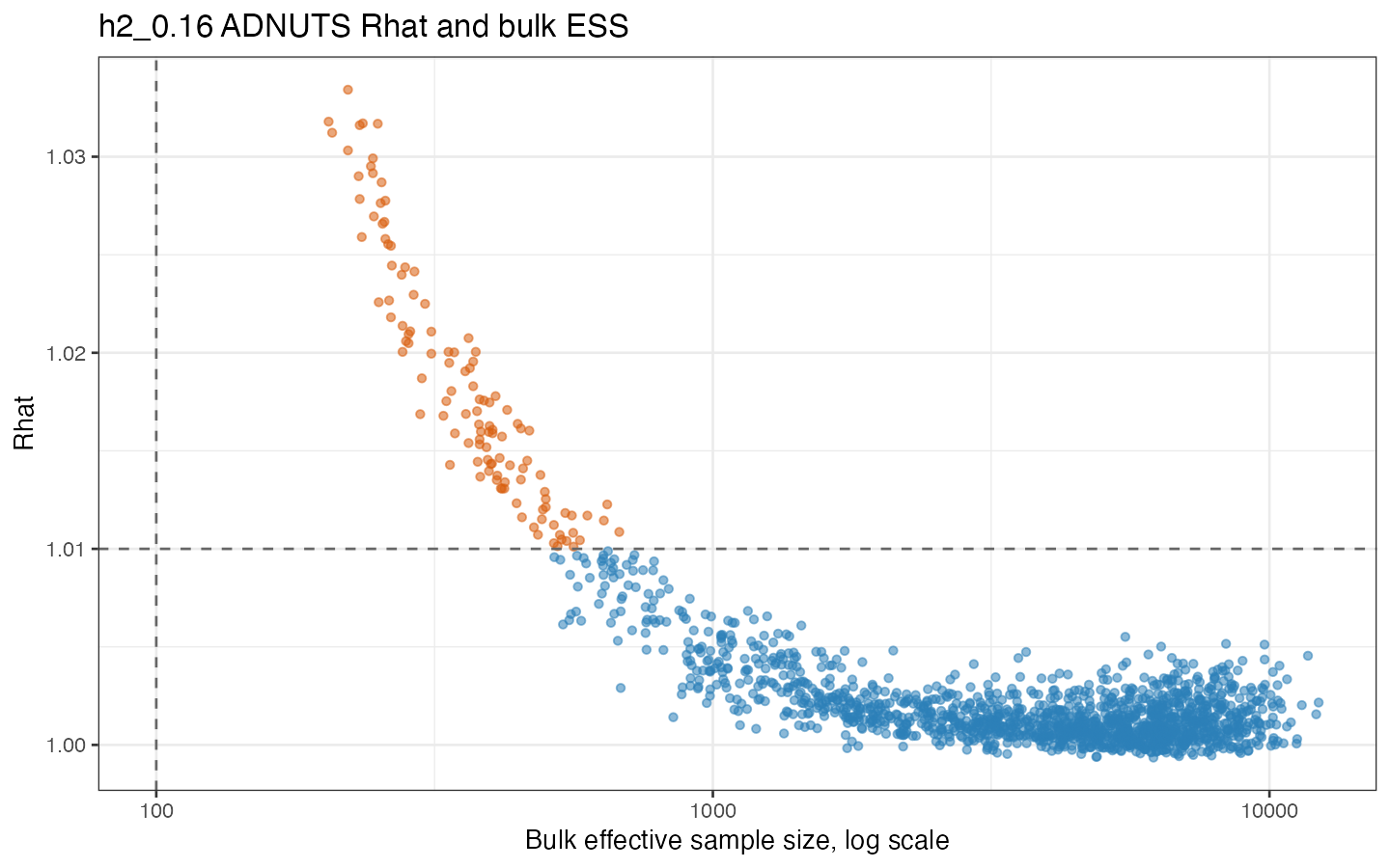
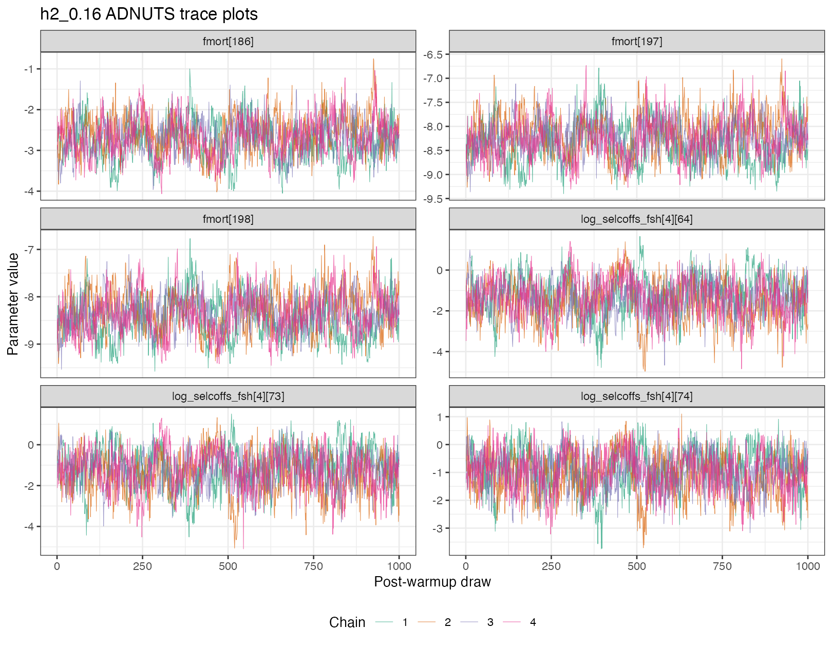
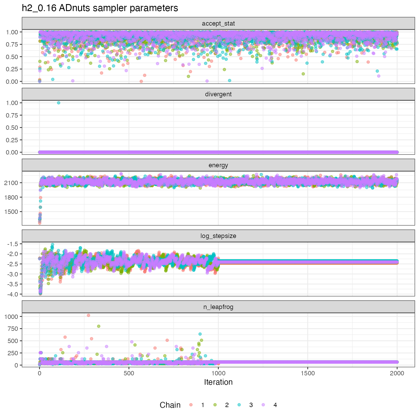
The diagnostics below use the base 0.16 development runs for the single-stock and two-stock hypotheses. Retrospective diagnostics use the standard five peels completed for h1_0.16 and h2_0.16. ADnuts MCMC diagnostics use four chains of 2,000 iterations, with 1,000 warmup iterations and 1,000 retained draws per chain.
h1_diag_nm <- "h1_0.16"
h2_diag_nm <- "h2_0.16"
h1_diag_model <- read_model_output(h1_diag_nm)
h2_diag_model <- read_model_output(h2_diag_nm)
h1_diag <- diagnostics(h1_diag_model, plot = FALSE)
h2_diag <- diagnostics(h2_diag_model, plot = FALSE)
source(file.path("R", "diagnostic_composition_plots.R"))
use_actual_model_ages <- function(selectivities) {
  if (!nrow(selectivities) || !"age" %in% names(selectivities)) {
    return(selectivities)
  }

  selectivities |>
    group_by(across(any_of(c(
      "model", "stock", "sel", "fleet_type", "fleet_number",
      "index", "year", "fleet_name"
    )))) |>
    arrange(.data$age, .by_group = TRUE) |>
    mutate(age = row_number()) |>
    ungroup()
}

selectivity_age_axis <- function(plot) {
  plot +
    scale_x_continuous(
      name = "Age",
      breaks = 1:12,
      limits = c(1, 12),
      minor_breaks = NULL,
      guide = guide_axis(check.overlap = TRUE, n.dodge = 2)
    )
}

h1_selectivities <- use_actual_model_ages(get_selectivities(h1_diag_model))
h2_selectivities <- use_actual_model_ages(get_selectivities(h2_diag_model))

adnuts_summary <- read_csv(file.path(doc_dir, "data", "adnuts_mcmc_summary.csv"), show_col_types = FALSE)
adnuts_slow <- read_csv(file.path(doc_dir, "data", "adnuts_mcmc_slow_parameters.csv"), show_col_types = FALSE)| Hypothesis | Model | Metric | Chains | Iterations | Warmup | Retained draws per chain | Divergences | Max tree-depth hits | Maximum Rhat | Minimum bulk ESS | Median bulk ESS |
|---|---|---|---|---|---|---|---|---|---|---|---|
| Single-stock | h1_0.16 | mle | 4 | 2000 | 1000 | 1000 | 1 | 52 | 1.043 | 71 | 2427.5 |
| Two-stock | h2_0.16 | mle | 4 | 2000 | 1000 | 1000 | 0 | 0 | 1.033 | 225 | 4134.0 |
| Model | Parameter | Bulk ESS | Rhat |
|---|---|---|---|
| h1_0.16 | log_selcoffs_fsh[4][118] | 71 | 1.035 |
| h1_0.16 | log_selcoffs_fsh[4][136] | 71 | 1.029 |
| h1_0.16 | log_selcoffs_fsh[4][127] | 72 | 1.033 |
| h1_0.16 | log_selcoffs_fsh[4][109] | 73 | 1.037 |
| h1_0.16 | log_selcoffs_fsh[4][73] | 77 | 1.043 |
| h1_0.16 | log_selcoffs_fsh[4][55] | 79 | 1.039 |
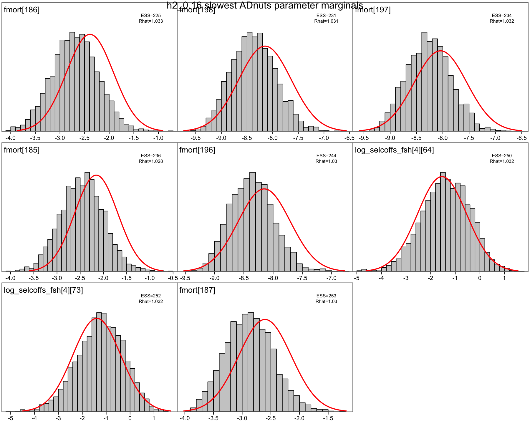
| h2_0.16 | fmort[186] | 225 | 1.033 |
| h2_0.16 | fmort[198] | 231 | 1.031 |
| h2_0.16 | fmort[197] | 234 | 1.032 |
| h2_0.16 | fmort[185] | 236 | 1.028 |
| h2_0.16 | fmort[196] | 244 | 1.030 |
| h2_0.16 | log_selcoffs_fsh[4][64] | 250 | 1.032 |
plot(h1_diag, var = "predictedObservedIndices")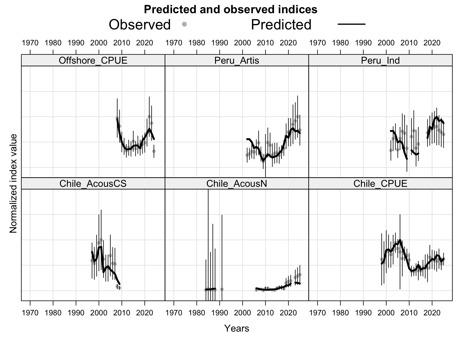
plot_catchability_diagnostics(h1_diag_model, model_label = h1_diag_nm)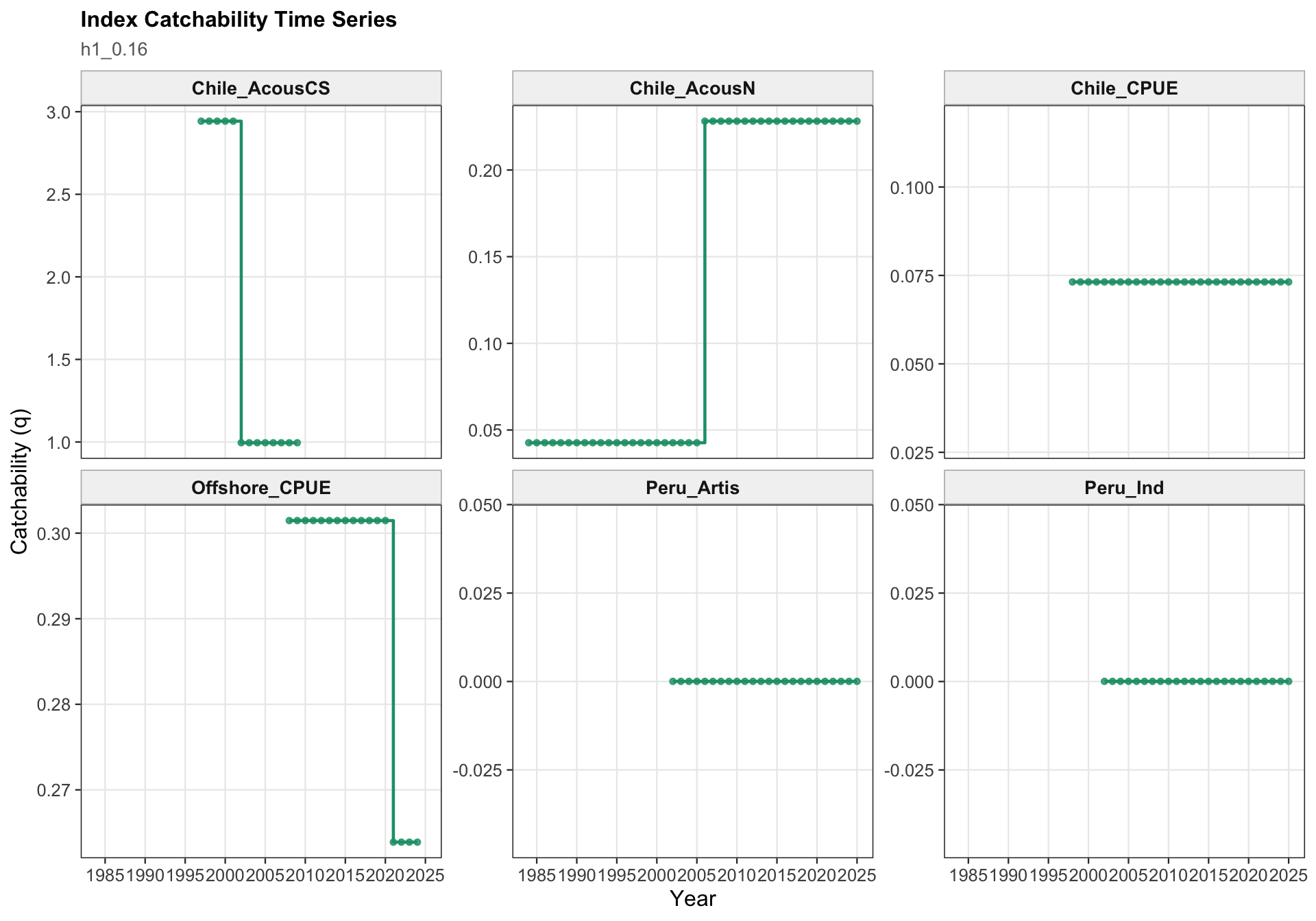
selectivity_age_axis(
  plot_selectivities(h1_selectivities, fleet = "fsh", alpha = 0.35, scale = 5)
)
selectivity_age_axis(
  plot_selectivities(h1_selectivities, fleet = "ind", alpha = 0.3, scale = 5)
)
h1_age_comp_fits <- diagnostic_comp_data(h1_diag_model, stock = 1, comp_type = "age") %>%
  filter(source_type == "fsh")
h1_age_comp_sources <- h1_age_comp_fits %>%
  distinct(source_id, source_name) %>%
  arrange(source_id) %>%
  pull(source_name)

walk(
  h1_age_comp_sources,
  ~print(plot_agecomp_fit(h1_age_comp_fits, .x, ncol = 4) + labs(subtitle = h1_diag_nm))
)
plot_composition_diagnostics(
  h1_diag_model,
  stock = 1,
  comp_type = "age",
  model_label = h1_diag_nm,
  exclude_source_pattern = "CPUE"
)
h1_length_comp_fits <- diagnostic_comp_data(h1_diag_model, stock = 1, comp_type = "length") %>%
  filter(source_type == "fsh")
h1_length_comp_sources <- h1_length_comp_fits %>%
  distinct(source_id, source_name) %>%
  arrange(source_id) %>%
  pull(source_name)

walk(
  h1_length_comp_sources,
  ~print(plot_lengthcomp_fit(h1_length_comp_fits, .x, ncol = 4) + labs(subtitle = h1_diag_nm))
)
plot_composition_diagnostics(
  h1_diag_model,
  stock = 1,
  comp_type = "length",
  model_label = h1_diag_nm,
  source_names = c("FarNorth")
)
load(file.path("results", paste0(h1_diag_nm, "_retrospective.RData")))
h1_retro <- output
plot(h1_retro, var = "SSB")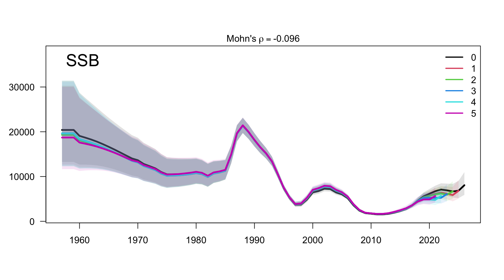
plot(h1_retro, var = "R")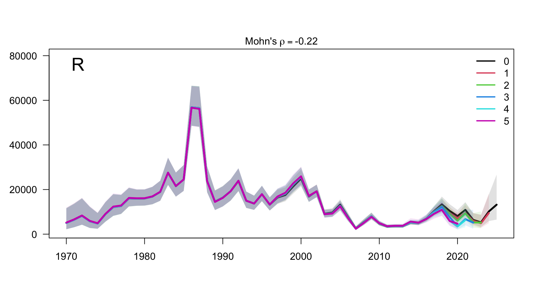
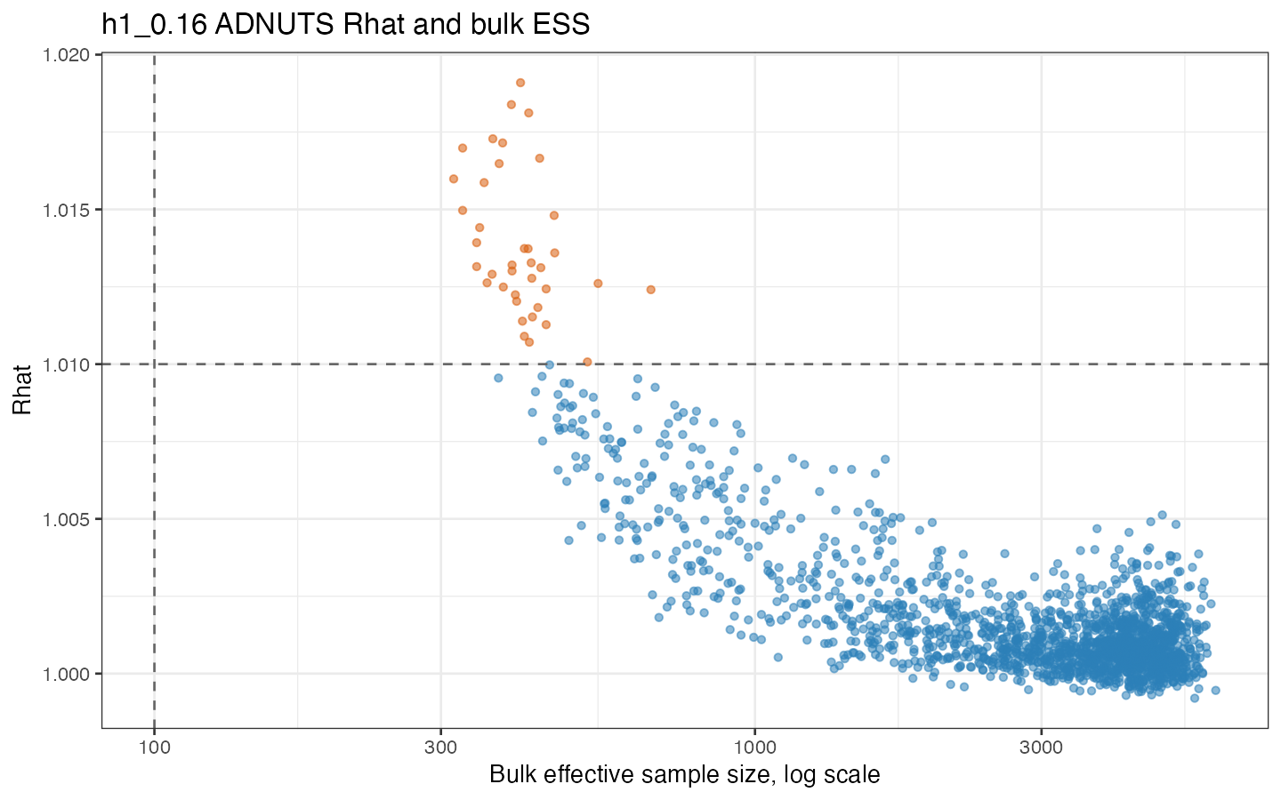
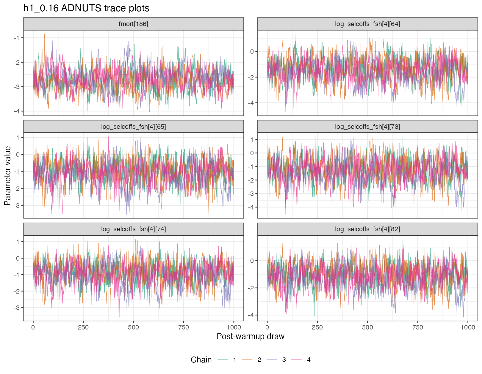
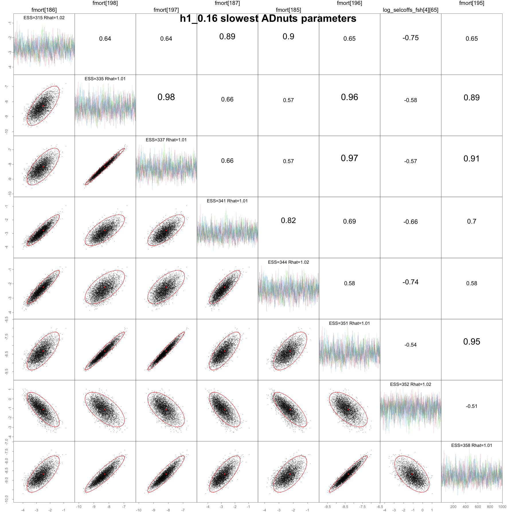
pairs_admb() plot for the eight slowest-mixing h1_0.16 parameters, with trace plots on the diagonal.
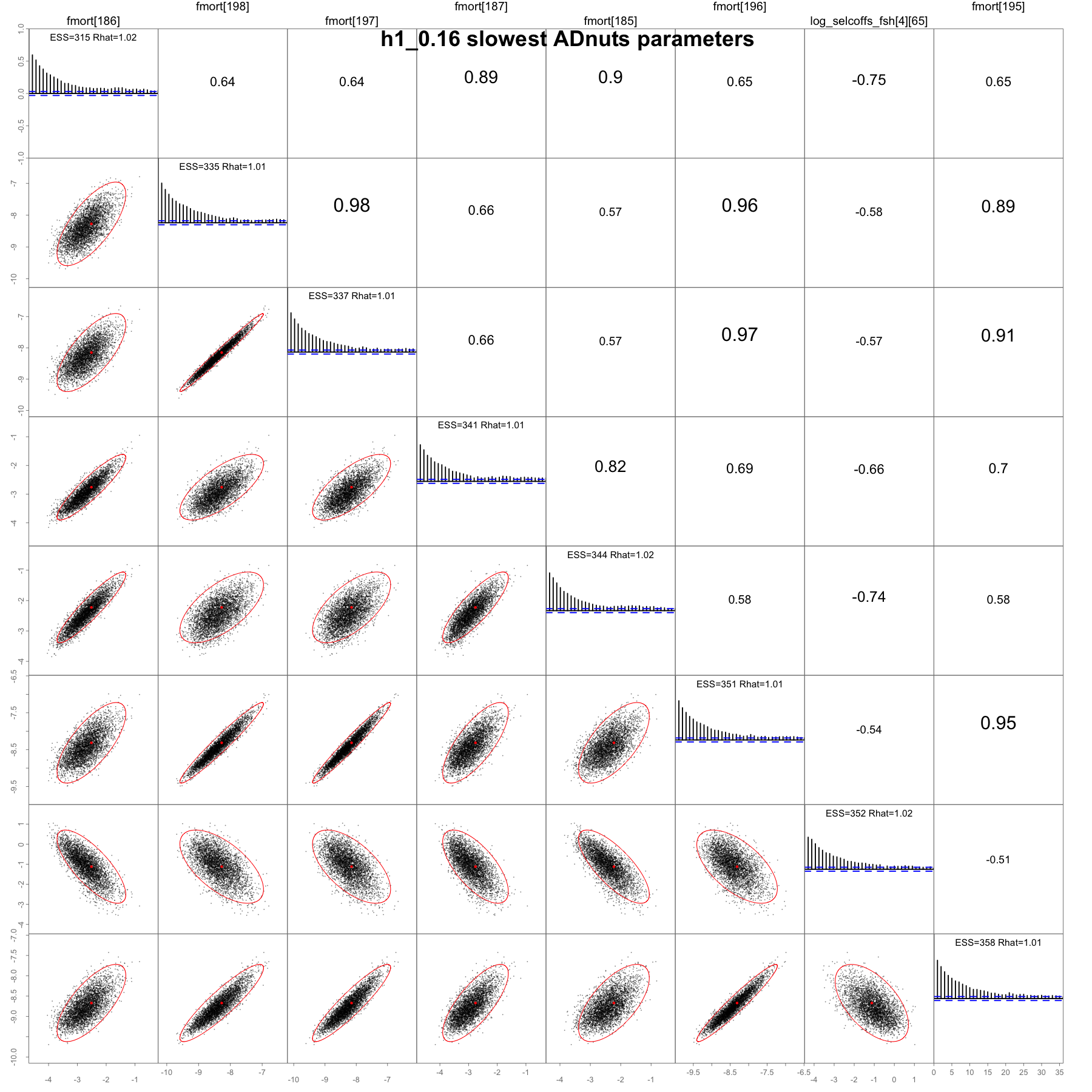
pairs_admb() plot for the eight slowest-mixing h1_0.16 parameters, with autocorrelation plots on the diagonal.
plot(h2_diag, var = "predictedObservedIndices")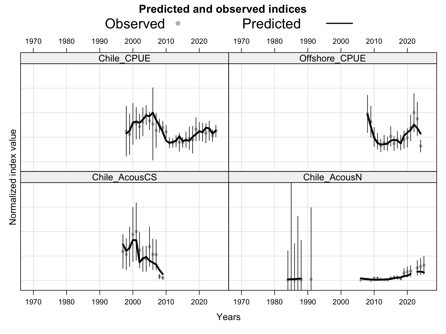
plot_catchability_diagnostics(h2_diag_model, model_label = h2_diag_nm)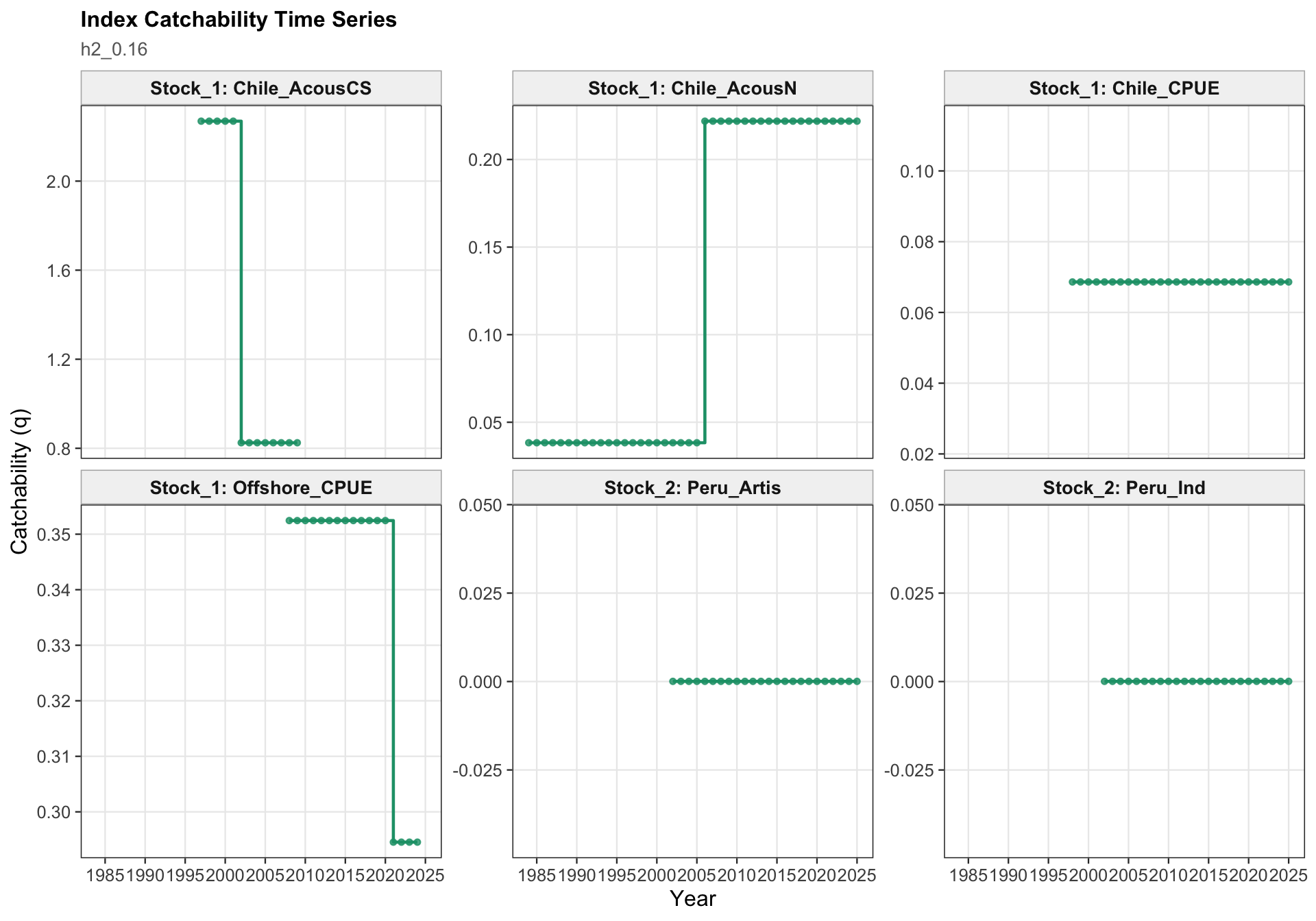
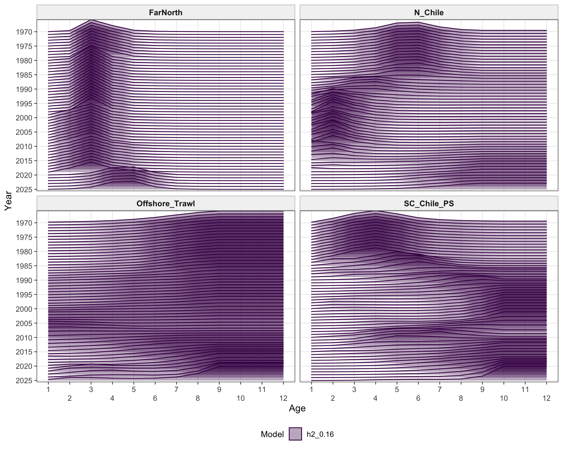
selectivity_age_axis(
  plot_selectivities(h2_selectivities, fleet = "fsh", alpha = 0.35, scale = 5)
)
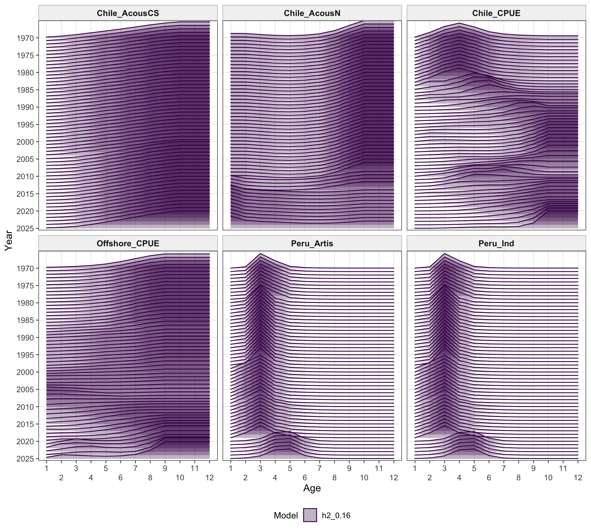
selectivity_age_axis(
  plot_selectivities(h2_selectivities, fleet = "ind", alpha = 0.3, scale = 5)
)
h2_age_comp_fits <- diagnostic_comp_data(h2_diag_model, stock = 1, comp_type = "age") %>%
  filter(source_type == "fsh")
h2_age_comp_sources <- h2_age_comp_fits %>%
  distinct(source_id, source_name) %>%
  arrange(source_id) %>%
  pull(source_name)

walk(
  h2_age_comp_sources,
  ~print(plot_agecomp_fit(h2_age_comp_fits, .x, ncol = 4) + labs(subtitle = paste(h2_diag_nm, "south stock")))
)
plot_composition_diagnostics(
  h2_diag_model,
  stock = 1,
  comp_type = "age",
  model_label = paste(h2_diag_nm, "south stock"),
  exclude_source_pattern = "CPUE"
)
h2_length_comp_fits <- diagnostic_comp_data(h2_diag_model, stock = 2, comp_type = "length") %>%
  filter(source_type == "fsh")
h2_length_comp_sources <- h2_length_comp_fits %>%
  distinct(source_id, source_name) %>%
  arrange(source_id) %>%
  pull(source_name)

walk(
  h2_length_comp_sources,
  ~print(plot_lengthcomp_fit(h2_length_comp_fits, .x, ncol = 4) + labs(subtitle = paste(h2_diag_nm, "FarNorth stock")))
)
plot_composition_diagnostics(
  h2_diag_model,
  stock = 2,
  comp_type = "length",
  model_label = paste(h2_diag_nm, "FarNorth stock"),
  source_names = c("FarNorth")
)
load(file.path("results", paste0(h2_diag_nm, "_retrospective.RData")))
h2_retro <- output
plot(h2_retro, var = "SSB")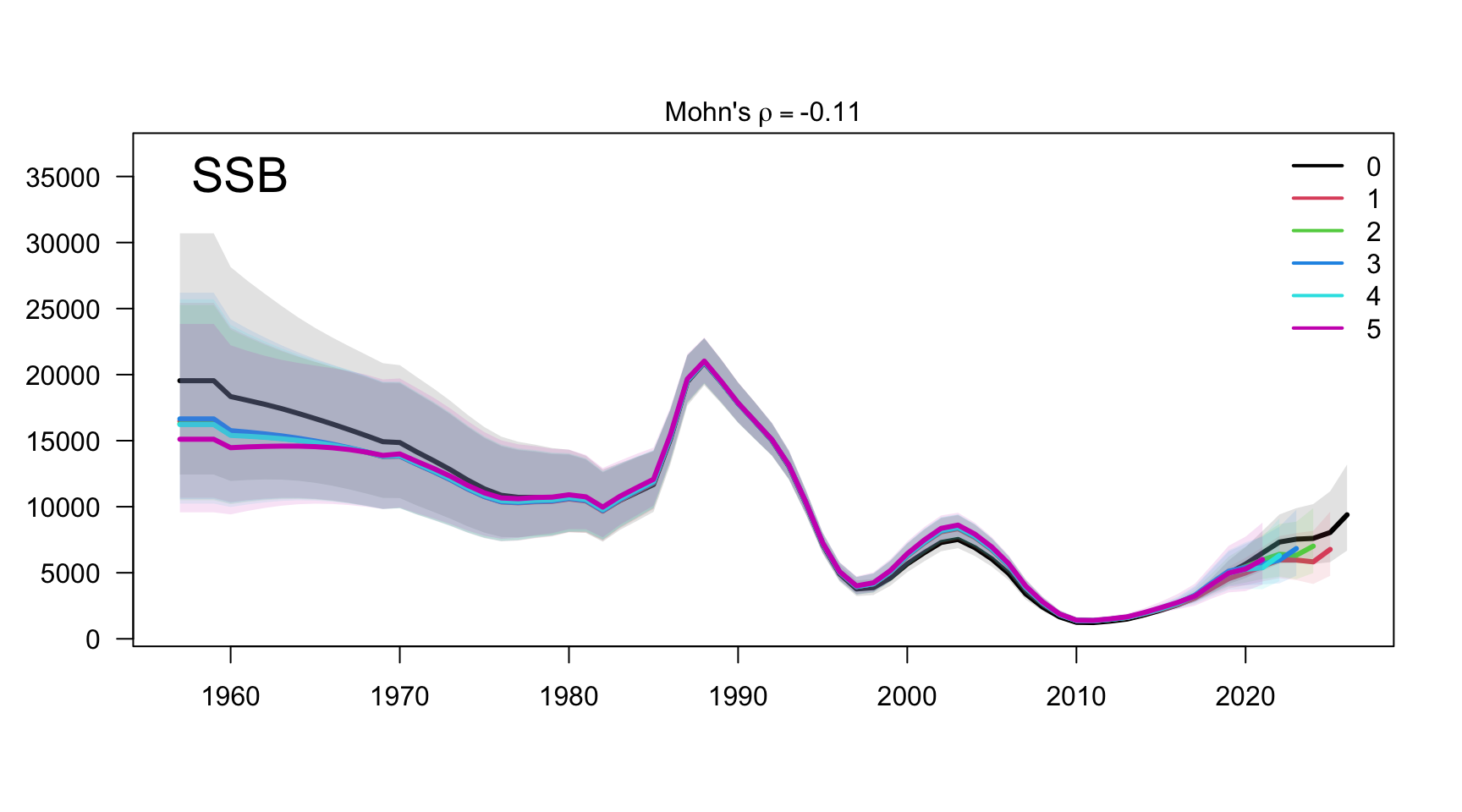
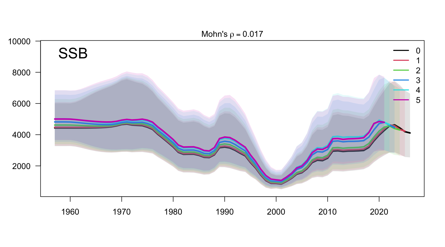
plot(h2_retro, var = "R")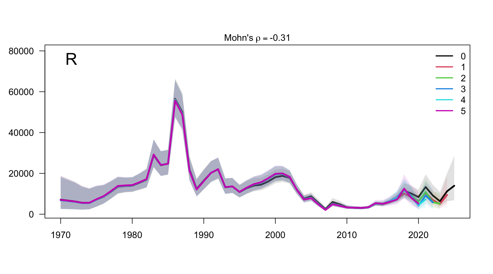
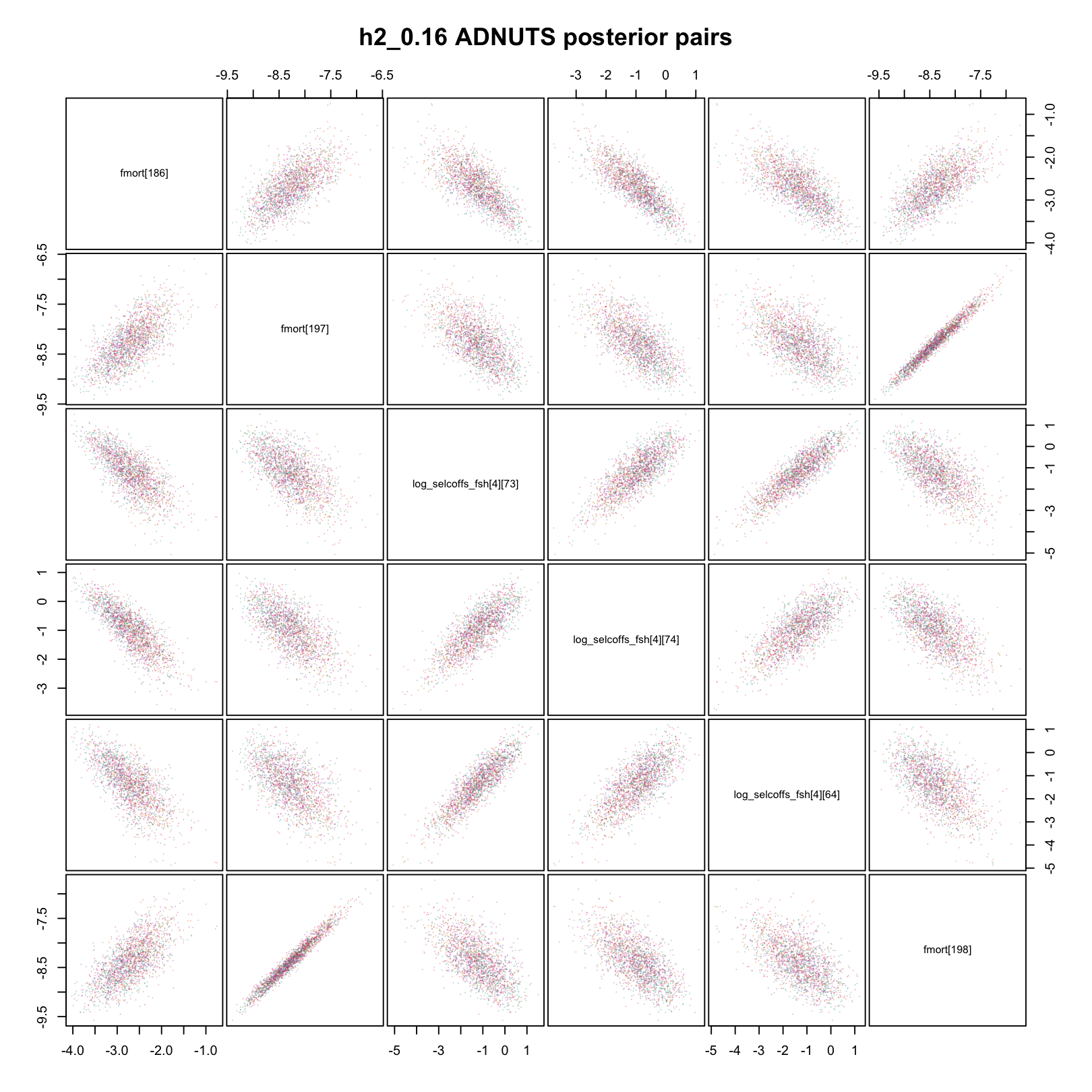
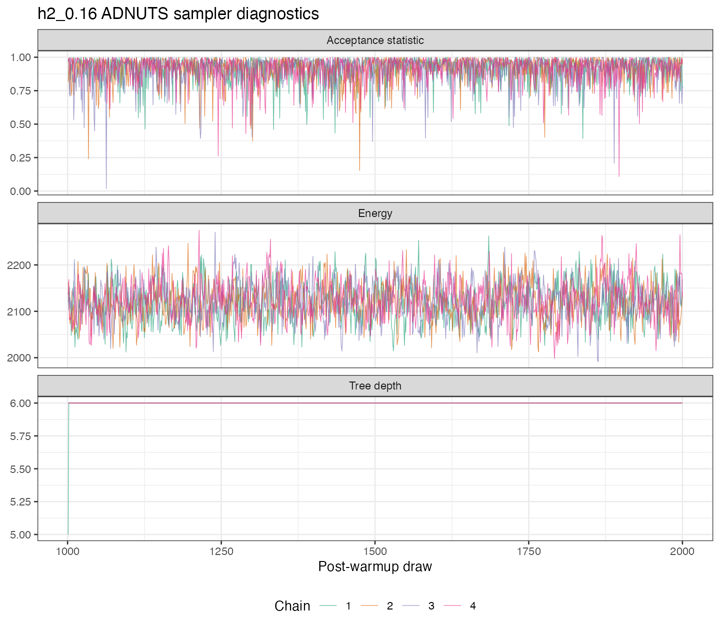
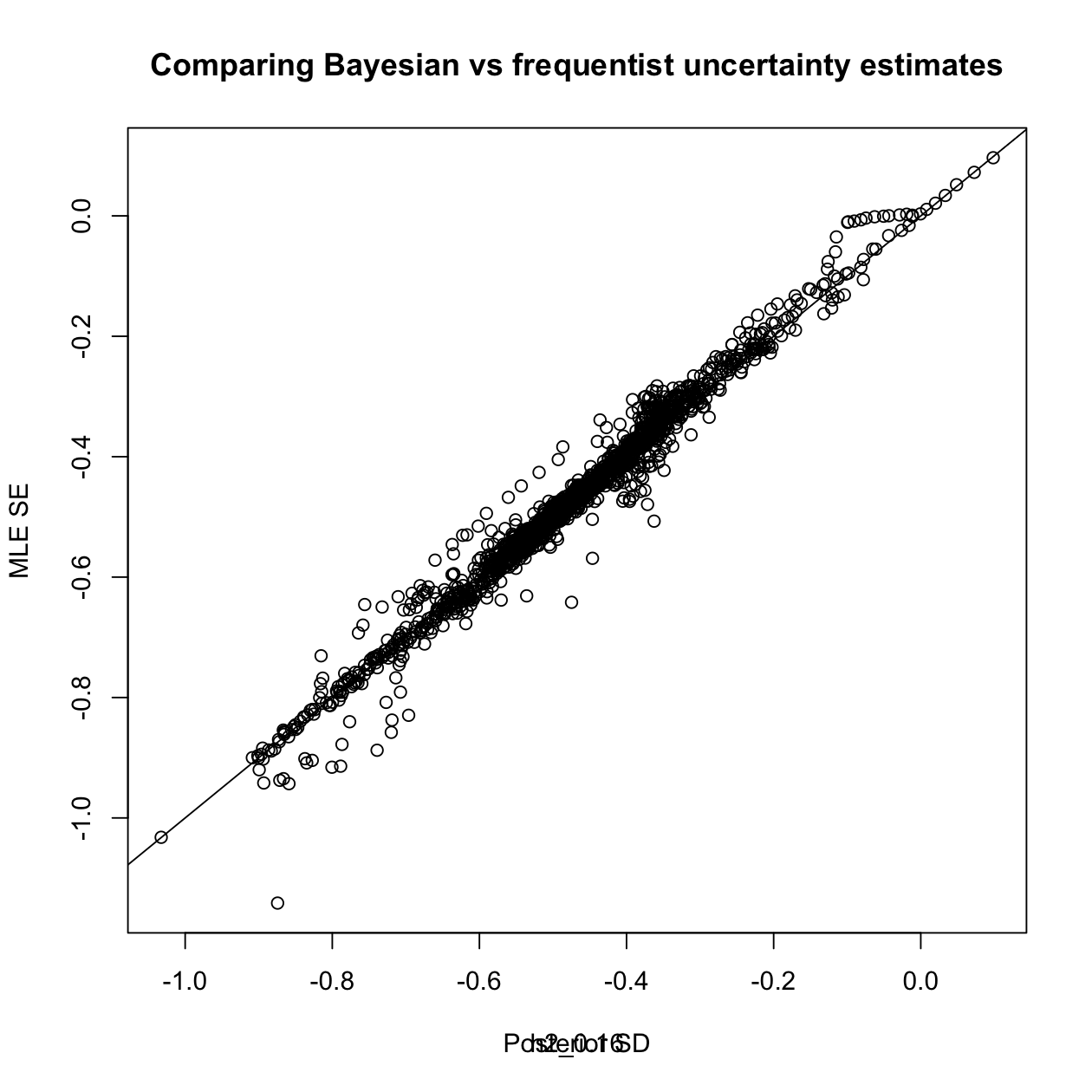
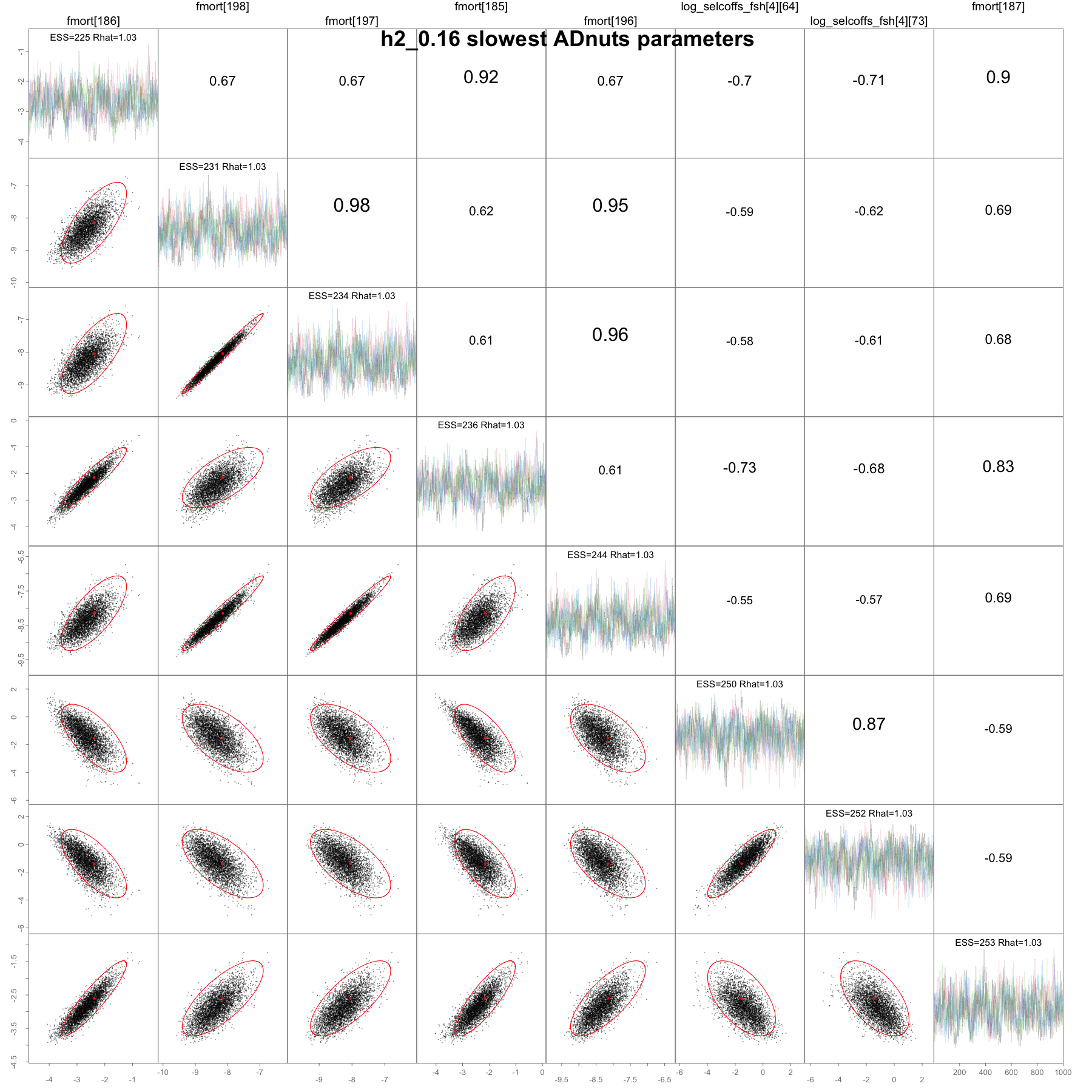
pairs_admb() plot for the eight slowest-mixing h2_0.16 parameters, with trace plots on the diagonal.
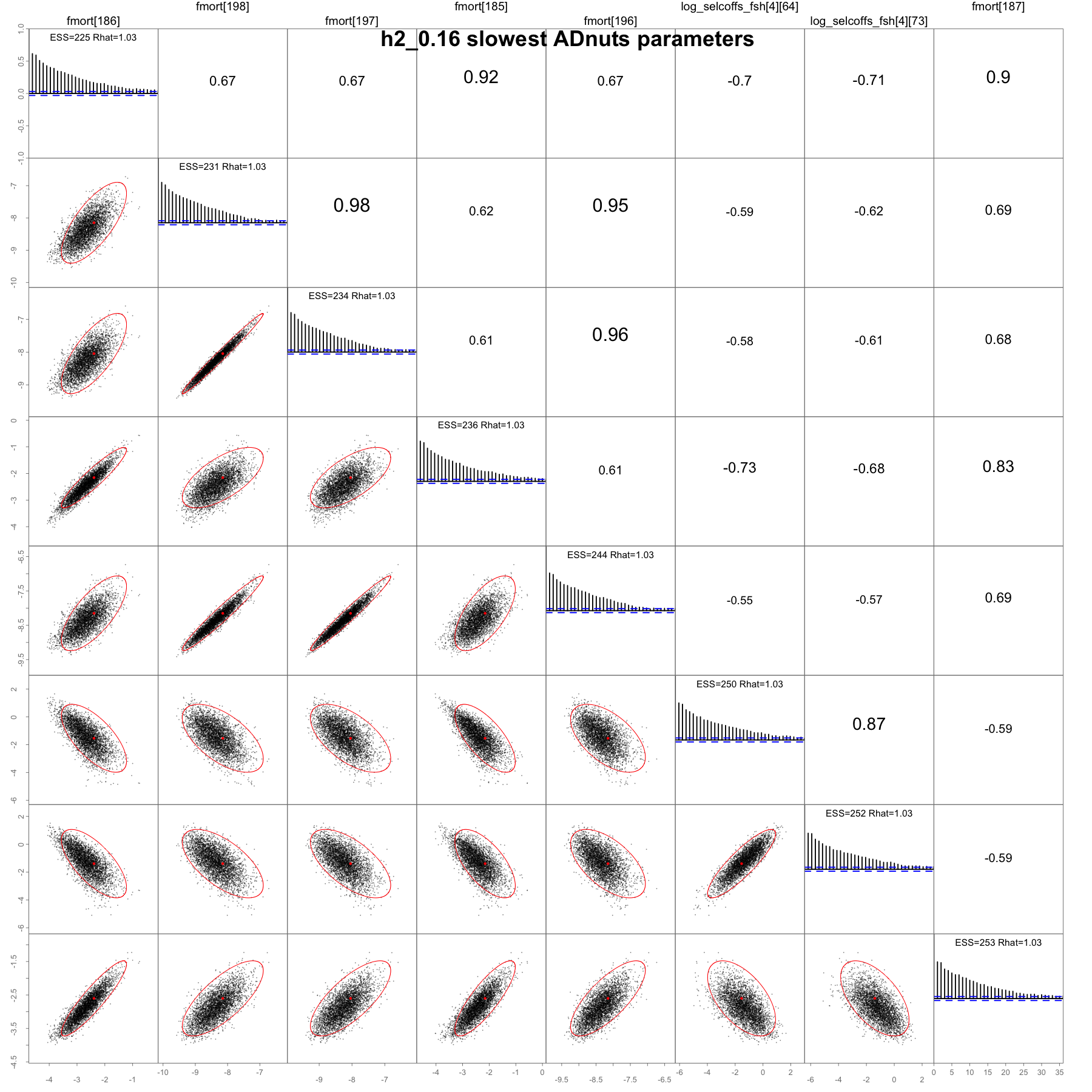
pairs_admb() plot for the eight slowest-mixing h2_0.16 parameters, with autocorrelation plots on the diagonal.
The current JJM template includes a smooth penalty on high average fishing mortality. For each stock and model year, total fishing mortality is first summed across fisheries for that stock. The intermediate value Fbar_tmp is the mean total F over ages 2-5. With Fcap = 3, eps = 0.05, and lambda_F = 10, the penalty contribution is:
\mathrm{excess} = {1 \over 2}\left[(Fbar\_tmp - Fcap) + \sqrt{(Fbar\_tmp - Fcap)^2 + eps^2}\right]
\mathrm{fpen} \mathrel{+}= \lambda_F \times \mathrm{excess}^2
This behaves like a differentiable approximation to 10 * max(0, Fbar_tmp - 3)^2. It is nearly zero below the cap, mild near Fbar_tmp = 3, and increasingly strong when a stock-year Fbar exceeds the cap. The form avoids a hard discontinuity in the objective function and is intended to discourage the unrealistically high terminal fishing-mortality spikes seen in some model-development trials without imposing a non-differentiable bound.
At render time, model outputs were available for the core bridge models 0.00, 0.14, 0.15, 0.16.