---
title: "Comparison of mod0.14 and mod0.5"
date: today
format:
  html:
    toc: true
    toc-depth: 3
    number-sections: true
    code-fold: true
    code-tools: true
    df-print: paged
    theme: cosmo
    fig-width: 9
    fig-height: 5
    lightbox: true
execute:
  warning: false
  message: false
---

```{r}
#| label: setup
#| include: false

assessment_dir <- normalizePath(
  Sys.getenv("JJM_ASSESSMENT_DIR", "/Users/jim/_mymods/sprfmo/jjm/assessment"),
  winslash = "/"
)
knitr::opts_knit$set(root.dir = assessment_dir)

library(jjmR)
library(dplyr)
library(ggplot2)
library(knitr)
library(purrr)
library(tidyr)

models <- c("mod0.14", "mod0.5")

read_par_summary <- function(model, output = file.path(assessment_dir, "results")) {
  vals <- as.numeric(scan(file.path(output, paste0(model, ".par")),
    what = "", n = 16, quiet = TRUE
  )[c(6, 11, 16)])

  tibble(
    model = model,
    n_parameters = as.integer(vals[[1]]),
    nll = vals[[2]],
    max_gradient = vals[[3]]
  )
}

read_model <- function(model) {
  readJJM(
    model,
    path = file.path(assessment_dir, "config"),
    input = file.path(assessment_dir, "input"),
    output = file.path(assessment_dir, "results"),
    version = "2015MS"
  )[[1]]
}

mods <- setNames(map(models, read_model), models)
fit_stats <- map_dfr(models, read_par_summary)

theme_report <- function() {
  theme_minimal(base_size = 12) +
    theme(
      legend.position = "top",
      panel.grid.minor = element_blank(),
      plot.title.position = "plot"
    )
}

series_df <- function(model, variable, label) {
  mat <- mods[[model]]$output[[1]][[variable]]
  colnames(mat) <- c("year", "estimate", "sd", "lower", "upper")
  as_tibble(mat) |>
    mutate(model = model, quantity = label)
}

survey_df <- function(model, survey_number) {
  survey <- mods[[model]]$output[[1]][[paste0("Obs_Survey_", survey_number)]]
  names <- mods[[model]]$data$Inames
  colnames(survey) <- c("year", "observed", "predicted", "se", "residual", "std_residual")
  as_tibble(survey) |>
    mutate(
      model = model,
      survey = names[[survey_number]]
    )
}

catch_df <- function(model) {
  out <- mods[[model]]$output[[1]]
  tibble(
    year = out$Yr,
    observed = out$Obs_catch_1,
    predicted = out$Pred_catch_1,
    model = model
  )
}

f_df <- function(model) {
  out <- mods[[model]]$output[[1]]
  as_tibble(out$TotF) |>
    mutate(year = out$Yr) |>
    pivot_longer(-year, names_to = "age", values_to = "f") |>
    mutate(
      model = model,
      age = as.integer(gsub("^V", "", age))
    )
}

like_df <- function(model) {
  out <- mods[[model]]$output[[1]]
  tibble(
    component = as.character(out$Like_Comp_names[, 1]),
    value = as.numeric(out$Like_Comp),
    model = model
  )
}

summary_df <- map_dfr(models, function(model) {
  data <- mods[[model]]$data
  control <- mods[[model]]$control
  tibble(
    model = model,
    data_file = control$dataFile,
    n_stocks = control$nStocks,
    n_fisheries = data$Fnum,
    fisheries = paste(data$Fnames, collapse = ", "),
    n_indices = data$Inum,
    indices = paste(data$Inames, collapse = ", "),
    start_year = data$years[[1]],
    end_year = data$years[[2]],
    min_age = data$ages[[1]],
    max_age = data$ages[[2]]
  )
})

bio_df <- map_dfr(models, \(model) bind_rows(
  series_df(model, "SSB", "Spawning biomass"),
  series_df(model, "TotBiom", "Total biomass"),
  series_df(model, "R", "Recruitment")
))

catch_comp <- map_dfr(models, catch_df)
survey_comp <- map_dfr(models, \(model) {
  map_dfr(seq_len(mods[[model]]$data$Inum), \(survey_number) {
    survey_df(model, survey_number)
  })
})
f_comp <- map_dfr(models, f_df)
like_comp <- map_dfr(models, like_df)
```

{{< include _includes/sprfmo-banner.html >}}

```{=html}
<div class="paper-title">Comparison of mod0.14 and mod0.5</div>
```

## Model Inputs

```{r}
#| label: tbl-model-inputs
#| tbl-cap: "Model input files and retained data sources."
#| echo: false

kable(summary_df, digits = 3)
```

```{r}
#| label: tbl-fit-stats
#| tbl-cap: "Model fit statistics read from the ADMB .par files."
#| echo: false

kable(fit_stats, digits = 5)
```

## Population Quantities

```{r}
#| label: fig-biomass-recruitment
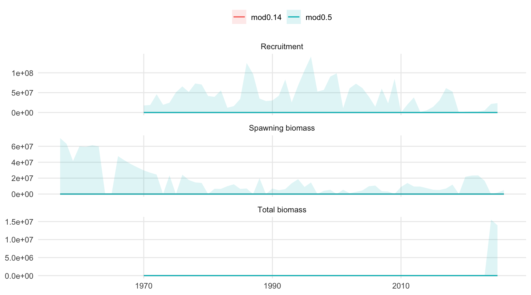
#| fig-cap: "Estimated population quantities. Ribbons show approximate uncertainty intervals from the JJM output."
#| echo: false

ggplot(bio_df, aes(year, estimate, color = model, fill = model)) +
  geom_ribbon(aes(ymin = lower, ymax = upper), alpha = 0.14, linewidth = 0) +
  geom_line(linewidth = 0.7) +
  facet_wrap(~quantity, scales = "free_y", ncol = 1) +
  labs(x = NULL, y = NULL, color = NULL, fill = NULL) +
  theme_report()
```

```{r}
#| label: fig-biomass-recruitment-post-1970
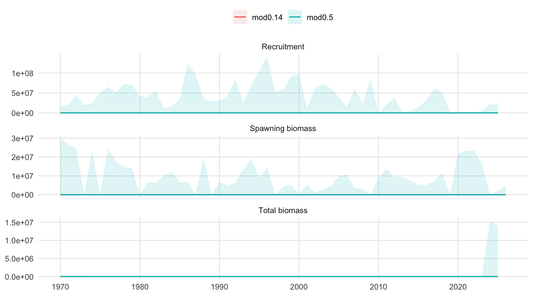
#| fig-cap: "Estimated population quantities from 1970 onward."
#| echo: false

bio_df |>
  filter(year >= 1970) |>
  ggplot(aes(year, estimate, color = model, fill = model)) +
  geom_ribbon(aes(ymin = lower, ymax = upper), alpha = 0.14, linewidth = 0) +
  geom_line(linewidth = 0.7) +
  facet_wrap(~quantity, scales = "free_y", ncol = 1) +
  labs(x = NULL, y = NULL, color = NULL, fill = NULL) +
  theme_report()
```

## Fishing Mortality

```{r}
#| label: fig-mean-f
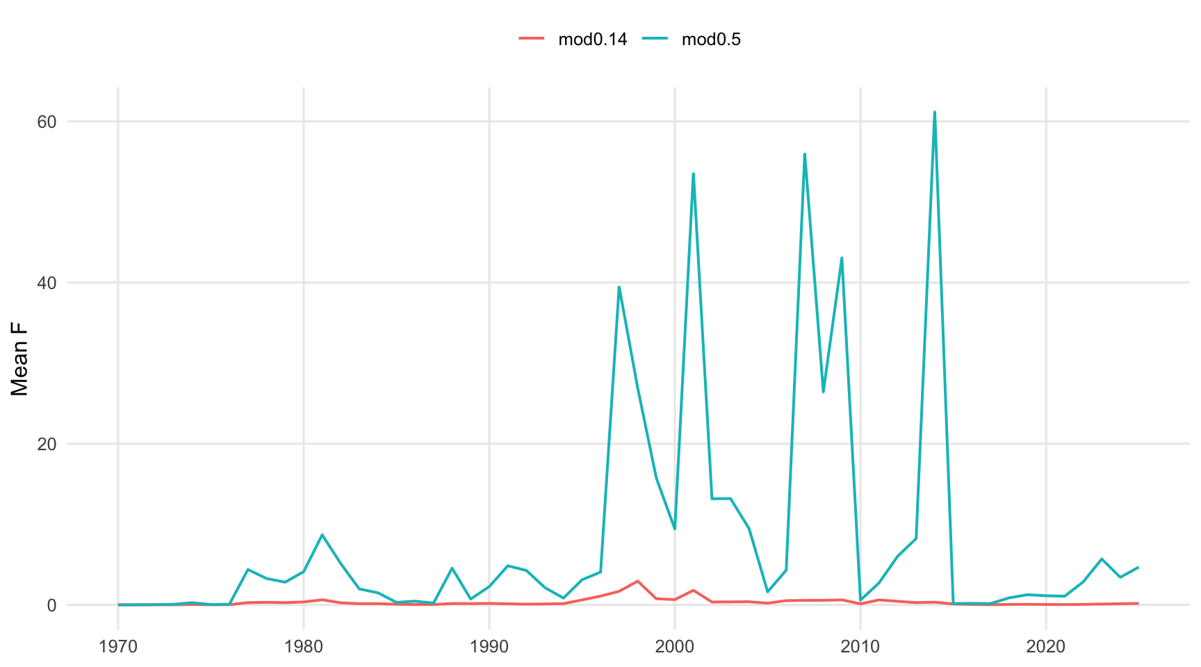
#| fig-cap: "Mean total fishing mortality across modeled ages."
#| echo: false

f_comp |>
  group_by(model, year) |>
  summarise(mean_f = mean(f, na.rm = TRUE), .groups = "drop") |>
  ggplot(aes(year, mean_f, color = model)) +
  geom_line(linewidth = 0.7) +
  labs(x = NULL, y = "Mean F", color = NULL) +
  theme_report()
```

```{r}
#| label: fig-f-by-age
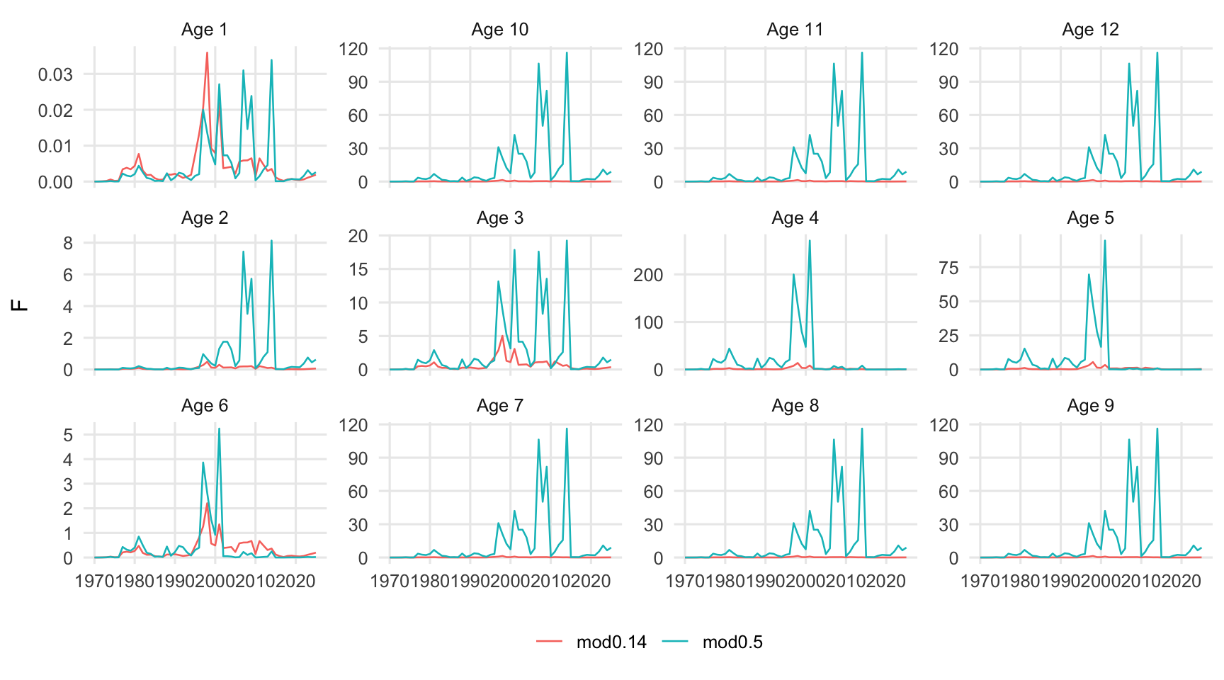
#| fig-cap: "Total fishing mortality by age."
#| echo: false

f_comp |>
  mutate(age = paste("Age", age)) |>
  ggplot(aes(year, f, color = model)) +
  geom_line(linewidth = 0.45) +
  facet_wrap(~age, scales = "free_y") +
  labs(x = NULL, y = "F", color = NULL) +
  theme_report() +
  theme(legend.position = "bottom")
```

## Fits To Data

```{r}
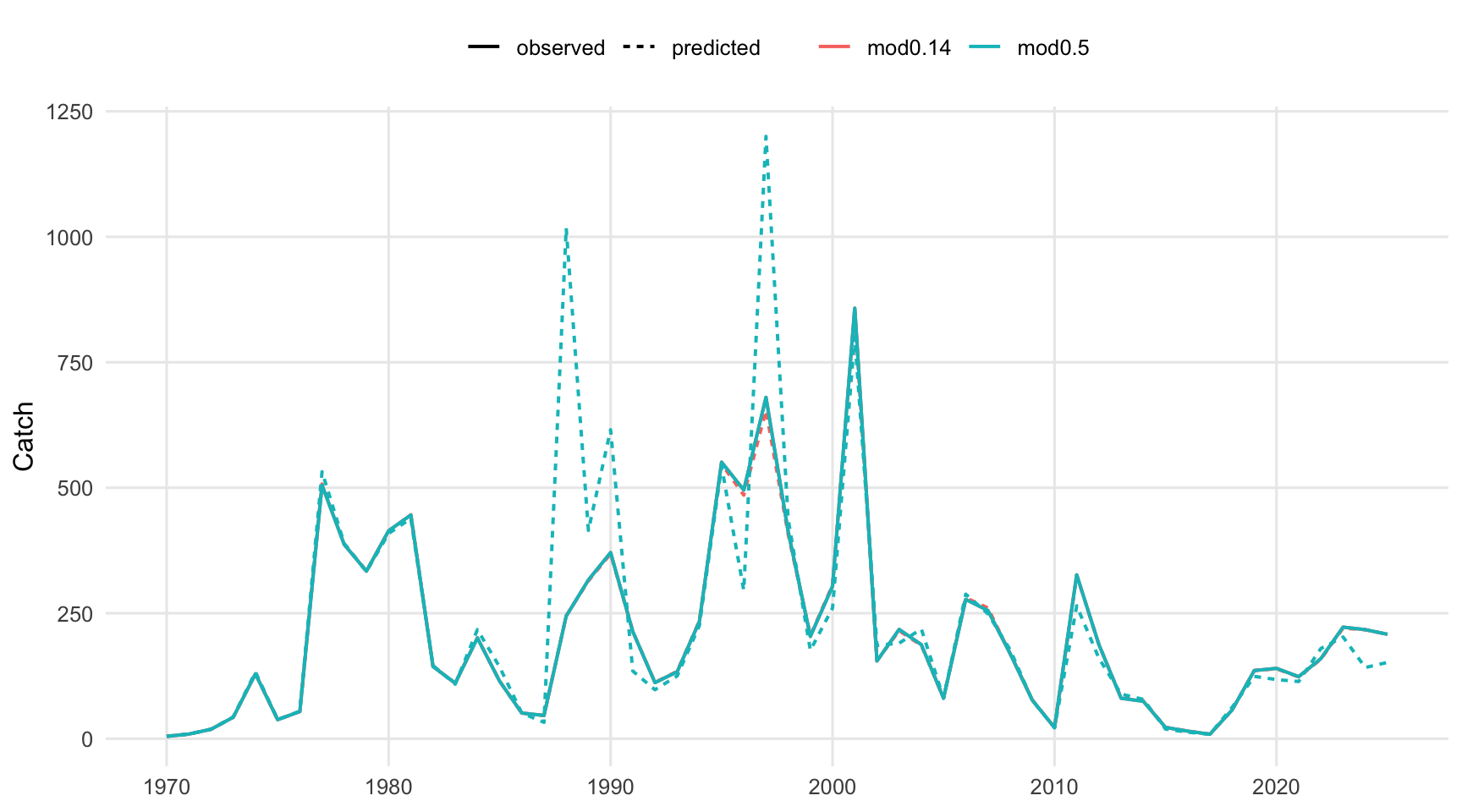
#| label: fig-catch-fit
#| fig-cap: "Observed and predicted catch for the FarNorth fishery."
#| echo: false

catch_comp |>
  pivot_longer(c(observed, predicted), names_to = "series", values_to = "catch") |>
  ggplot(aes(year, catch, color = model, linetype = series)) +
  geom_line(linewidth = 0.7) +
  labs(x = NULL, y = "Catch", color = NULL, linetype = NULL) +
  theme_report()
```

```{r}
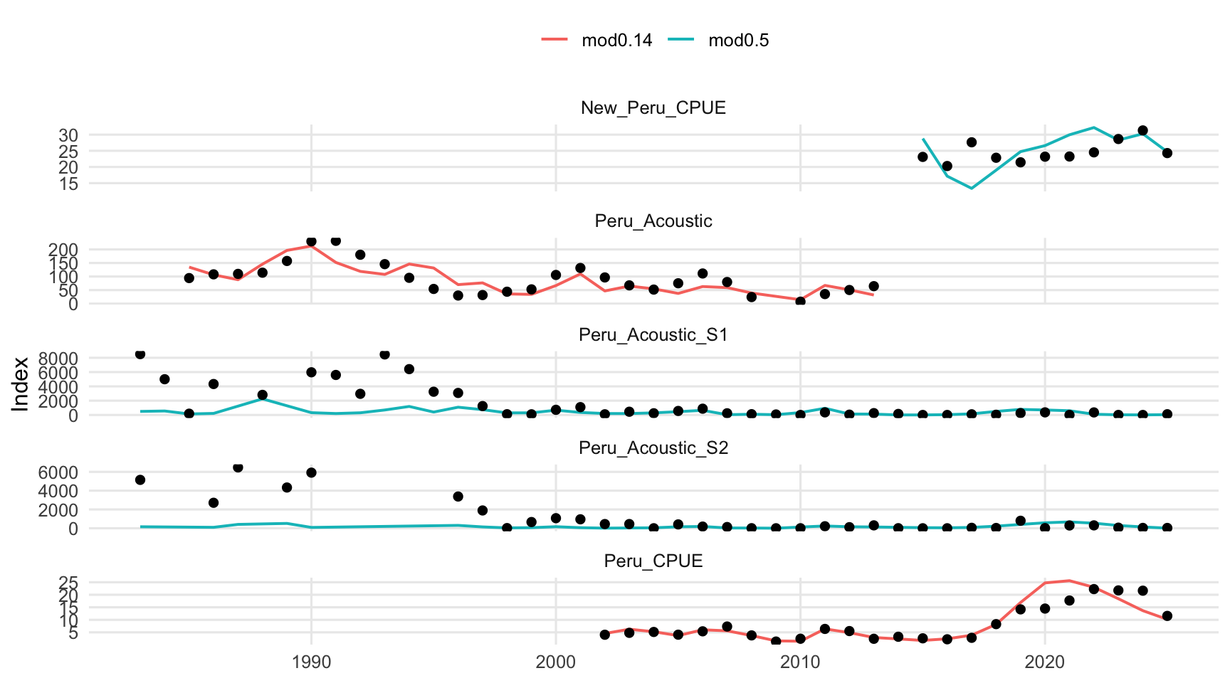
#| label: fig-survey-fit
#| fig-cap: "Observed and predicted indices for the retained Peru survey and CPUE series."
#| echo: false

survey_obs <- survey_comp |>
  distinct(survey, year, observed)

ggplot(survey_comp, aes(year, predicted, color = model)) +
  geom_line(linewidth = 0.7) +
  geom_point(
    data = survey_obs,
    aes(year, observed),
    inherit.aes = FALSE,
    color = "black",
    size = 1.8
  ) +
  facet_wrap(~survey, scales = "free_y", ncol = 1) +
  labs(x = NULL, y = "Index", color = NULL) +
  theme_report()
```

## Likelihood Components

```{r}
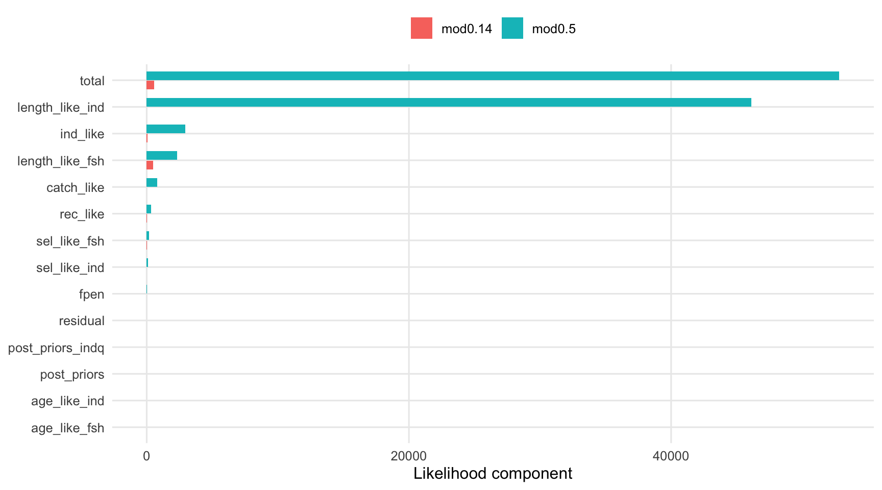
#| label: fig-likelihood-components
#| fig-cap: "Likelihood components by model."
#| echo: false

ggplot(like_comp, aes(reorder(component, value), value, fill = model)) +
  geom_col(position = position_dodge(width = 0.7), width = 0.65) +
  coord_flip() +
  labs(x = NULL, y = "Likelihood component", fill = NULL) +
  theme_report()
```

```{r}
#| label: tbl-likelihood-components
#| tbl-cap: "Likelihood component values."
#| echo: false

like_comp |>
  pivot_wider(names_from = model, values_from = value) |>
  kable(digits = 3)
```