---
title: "Kobe Plot Alternatives for Model 0.14"
date: today
format:
  html:
    toc: true
    toc-depth: 2
    code-fold: true
    code-tools: true
    df-print: paged
    theme: cosmo
    fig-width: 9
    fig-height: 5
    lightbox: true
execute:
  warning: false
  message: false
params:
  model_name: "h1_0.14"
  stock: 1
---

```{r}
#| label: setup
#| include: false

library(jjmR)
library(dplyr)
library(ggplot2)
library(knitr)
library(tidyr)

assessment_dir <- normalizePath(file.path("..", "assessment"), mustWork = TRUE)
assessment_file <- function(...) file.path(assessment_dir, ...)

read_model <- function(model_name) {
  readJJM(
    model_name,
    path = assessment_file("config"),
    input = assessment_file("input"),
    output = assessment_file("results"),
    version = "2015MS"
  )[[1]]
}

theme_report <- function() {
  theme_minimal(base_size = 12) +
    theme(
      legend.position = "top",
      panel.grid.minor = element_blank(),
      plot.title.position = "plot"
    )
}

as_estimate_df <- function(x, quantity = NULL) {
  out <- as_tibble(x)
  names(out) <- c("year", "estimate", "sd", "lower", "upper")
  out <- mutate(out, across(everything(), as.numeric))
  if (!is.null(quantity)) {
    out <- mutate(out, quantity = quantity, .before = 1)
  }
  out
}

read_yield_profile <- function(model_name) {
  yld_file <- assessment_file("results", paste0(model_name, ".yld"))
  read.table(
    yld_file,
    skip = 5,
    fill = TRUE,
    col.names = c("f", "spawning_biomass", "yield", "recruitment", "spr", "total_biomass")
  ) |>
    as_tibble() |>
    filter(!is.na(f), !is.na(spr)) |>
    mutate(across(everything(), as.numeric))
}

read_std_terms <- function(model_name, terms) {
  std_file <- assessment_file("results", paste0(model_name, ".std"))
  out <- tibble(
    term = terms,
    value = NA_real_,
    std_dev = NA_real_
  )

  if (!file.exists(std_file)) {
    return(out)
  }

  std_output <- read.table(std_file, header = TRUE)
  matched <- match(terms, std_output$name)
  out$value <- as.numeric(std_output$value[matched])
  out$std_dev <- as.numeric(std_output$std.dev[matched])
  out
}

read_std_value <- function(model_name, term) {
  read_std_terms(model_name, term)$value[[1]]
}

read_r_report_value <- function(model_name, term) {
  r_report_file <- assessment_file("results", paste0(model_name, "_1_R.rep"))
  if (!file.exists(r_report_file)) {
    return(NA_real_)
  }

  r_report <- readLines(r_report_file, warn = FALSE)
  term_line <- which(r_report == paste0("$", term))[1]
  if (is.na(term_line) || term_line == length(r_report)) {
    return(NA_real_)
  }

  as.numeric(strsplit(trimws(r_report[term_line + 1]), "\\s+")[[1]][1])
}

interpolate_spr <- function(profile, target_spr = 0.35) {
  profile <- arrange(profile, f)
  crossing <- which(
    (head(profile$spr, -1) - target_spr) *
      (tail(profile$spr, -1) - target_spr) <= 0
  )[1]

  if (is.na(crossing)) {
    return(tibble(
      profile_f_at_spr35 = NA_real_,
      sbf35 = NA_real_,
      yield_at_spr35 = NA_real_,
      recruitment_at_spr35 = NA_real_,
      total_biomass_at_spr35 = NA_real_
    ))
  }

  lower <- profile[crossing, ]
  upper <- profile[crossing + 1, ]
  weight <- (target_spr - lower$spr) / (upper$spr - lower$spr)

  tibble(
    profile_f_at_spr35 = lower$f + weight * (upper$f - lower$f),
    sbf35 = lower$spawning_biomass + weight * (upper$spawning_biomass - lower$spawning_biomass),
    yield_at_spr35 = lower$yield + weight * (upper$yield - lower$yield),
    recruitment_at_spr35 = lower$recruitment + weight * (upper$recruitment - lower$recruitment),
    total_biomass_at_spr35 = lower$total_biomass + weight * (upper$total_biomass - lower$total_biomass)
  )
}

interpolate_f <- function(profile, target_f) {
  if (!is.finite(target_f)) {
    return(tibble(
      spawning_biomass_at_f = NA_real_,
      yield_at_f = NA_real_,
      recruitment_at_f = NA_real_,
      spr_at_f = NA_real_,
      total_biomass_at_f = NA_real_
    ))
  }

  profile <- arrange(profile, f)
  tibble(
    spawning_biomass_at_f = approx(profile$f, profile$spawning_biomass, xout = target_f)$y,
    yield_at_f = approx(profile$f, profile$yield, xout = target_f)$y,
    recruitment_at_f = approx(profile$f, profile$recruitment, xout = target_f)$y,
    spr_at_f = approx(profile$f, profile$spr, xout = target_f)$y,
    total_biomass_at_f = approx(profile$f, profile$total_biomass, xout = target_f)$y
  )
}

model <- read_model(params$model_name)
stock_output <- model$output[[params$stock]]
yield_profile <- read_yield_profile(params$model_name)
profile_fmsy <- yield_profile$f[which.max(yield_profile$yield)]
reported_fmsy <- read_std_value(params$model_name, "Fmsy")
fmsy <- if (is.finite(reported_fmsy)) reported_fmsy else profile_fmsy

productivity_models <- tibble(
  model = c(params$model_name, "h1_0.14ll", "h1_0.14hl", "h1_0.14hs"),
  scenario = c(
    "Low steepness, short SR",
    "Low steepness, long SR",
    "High steepness, long SR",
    "High steepness, short SR"
  ),
  steepness = c(0.65, 0.65, 0.85, 0.85),
  sr_fit = c("Short", "Long", "Long", "Short"),
  sr_years = c("2000-2022", "1970-2022", "1970-2022", "2000-2022")
)

summarize_productivity_model <- function(model_name) {
  profile <- read_yield_profile(model_name)
  profile_msy_row <- profile[which.max(profile$yield), ]
  std_terms <- read_std_terms(model_name, c("Fmsy", "Fcur_Fmsy", "Bmsy", "Bcur_Bmsy"))
  spr35 <- interpolate_spr(profile, target_spr = 0.35)

  tibble(
    model = model_name,
    Fmsy = std_terms$value[std_terms$term == "Fmsy"],
    Fmsy_se = std_terms$std_dev[std_terms$term == "Fmsy"],
    F35_est = read_r_report_value(model_name, "F35_est"),
    F_at_SPR35_profile = spr35$profile_f_at_spr35,
    Fcur_Fmsy = std_terms$value[std_terms$term == "Fcur_Fmsy"],
    Bmsy = std_terms$value[std_terms$term == "Bmsy"],
    Bmsy_se = std_terms$std_dev[std_terms$term == "Bmsy"],
    Bcur_Bmsy = std_terms$value[std_terms$term == "Bcur_Bmsy"],
    profile_Fmsy = profile_msy_row$f,
    MSY = profile_msy_row$yield,
    SPR_at_profile_Fmsy = profile_msy_row$spr
  )
}

productivity_reference <- bind_rows(
  lapply(productivity_models$model, summarize_productivity_model)
) |>
  left_join(productivity_models, by = "model") |>
  mutate(
    Fmsy_lower = pmax(Fmsy - 1.96 * Fmsy_se, 0),
    Fmsy_upper = Fmsy + 1.96 * Fmsy_se
  ) |>
  arrange(Fmsy) |>
  mutate(
    scenario = factor(scenario, levels = scenario),
    sr_fit = factor(sr_fit, levels = c("Short", "Long")),
    steepness_label = factor(
      paste0("h = ", steepness),
      levels = c("h = 0.65", "h = 0.85")
    )
  )

productivity_yield_profiles <- bind_rows(
  lapply(productivity_models$model, \(model_name) {
    read_yield_profile(model_name) |>
      mutate(model = model_name, .before = 1)
  })
) |>
  left_join(
    productivity_reference |>
      select(model, scenario, steepness_label, sr_fit),
    by = "model"
  )

productivity_f_reference_points <- productivity_reference |>
  select(model, scenario, steepness_label, sr_fit, Fmsy, F35_est) |>
  pivot_longer(
    cols = c(Fmsy, F35_est),
    names_to = "reference",
    values_to = "f"
  ) |>
  mutate(
    reference = recode(reference, Fmsy = "Fmsy", F35_est = "F35%"),
    reference = factor(reference, levels = c("Fmsy", "F35%"))
  )

bmsy_reference <- productivity_reference |>
  transmute(
    model,
    scenario,
    Bmsy,
    Bmsy_se,
    Bcur_Bmsy,
    bmsy_label = factor(
      recode(
        as.character(scenario),
        "Low steepness, short SR" = "low h, short",
        "Low steepness, long SR" = "low h, long",
        "High steepness, short SR" = "high h, short",
        "High steepness, long SR" = "high h, long"
      ),
      levels = c("low h, short", "low h, long", "high h, short", "high h, long")
    )
  )

read_productivity_ssb <- function(model_name) {
  model_obj <- if (identical(model_name, params$model_name)) model else read_model(model_name)
  stock_obj <- model_obj$output[[params$stock]]
  ssb <- as_tibble(stock_obj$df1)
  names(ssb) <- c("quantity", "year", "estimate", "sd", "lower", "upper")

  ssb |>
    mutate(across(-quantity, as.numeric)) |>
    filter(quantity == "SSB") |>
    mutate(model = model_name, .before = 1)
}

productivity_ssb_series <- bind_rows(
  lapply(productivity_models$model, read_productivity_ssb)
) |>
  left_join(
    productivity_models |>
      select(model, scenario),
    by = "model"
  ) |>
  mutate(
    scenario = factor(scenario, levels = levels(productivity_reference$scenario))
  )

productivity_scenario_colors <- c(
  "Low steepness, short SR" = "#2c7fb8",
  "Low steepness, long SR" = "#74a9cf",
  "High steepness, long SR" = "#d95f0e",
  "High steepness, short SR" = "#fdb863"
)

read_productivity_majuro <- function(model_name) {
  model_obj <- if (identical(model_name, params$model_name)) model else read_model(model_name)
  stock_obj <- model_obj$output[[params$stock]]
  f_names <- grep("^F_fsh_[0-9]+$", names(stock_obj), value = TRUE)

  annual_f <- bind_rows(
    lapply(f_names, \(name) {
      values <- as_tibble(stock_obj[[name]], .name_repair = "minimal")
      names(values) <- c("year", "mean_f", "max_selectivity_scaled_f")
      values
    })
  ) |>
    mutate(across(everything(), as.numeric)) |>
    group_by(year) |>
    summarize(f = sum(mean_f), .groups = "drop")

  depletion <- as_estimate_df(stock_obj$SSB_NoFishR, "SSB_NoFishR") |>
    select(year, depletion = estimate, depletion_lower = lower, depletion_upper = upper)

  depletion |>
    left_join(annual_f, by = "year") |>
    mutate(
      model = model_name,
      f_fmsy = f / productivity_reference$Fmsy[match(model_name, productivity_reference$model)],
      .before = 1
    )
}

majuro_series <- bind_rows(
  lapply(productivity_models$model, read_productivity_majuro)
) |>
  left_join(
    productivity_models |>
      select(model, scenario),
    by = "model"
  ) |>
  mutate(
    scenario = factor(scenario, levels = levels(productivity_reference$scenario))
  )

majuro_terminal <- majuro_series |>
  group_by(model, scenario) |>
  filter(year == max(year)) |>
  ungroup()

majuro_x_upper <- max(0.6, ceiling(max(majuro_series$depletion[majuro_series$year >= 2000], na.rm = TRUE) * 10) / 10)
majuro_y_upper <- max(1.2, ceiling(max(majuro_series$f_fmsy[majuro_series$year >= 2000], na.rm = TRUE) * 10) / 10)

df1 <- as_tibble(stock_output$df1)
names(df1) <- c("quantity", "year", "estimate", "sd", "lower", "upper")
df1 <- df1 |>
  mutate(across(-quantity, as.numeric))

biomass_series <- df1 |>
  filter(quantity %in% c(
    "SSB",
    "SSB_Nofishing",
    "Total_Biom",
    "Total_Biom_Nofishing"
  )) |>
  mutate(
    metric = case_when(
      quantity %in% c("SSB", "SSB_Nofishing") ~ "Spawning biomass",
      quantity %in% c("Total_Biom", "Total_Biom_Nofishing") ~ "Total biomass"
    ),
    scenario = case_when(
      quantity %in% c("SSB", "Total_Biom") ~ "With fishing",
      quantity %in% c("SSB_Nofishing", "Total_Biom_Nofishing") ~ "Without fishing"
    )
  ) |>
  select(metric, scenario, year, estimate, sd, lower, upper)

biomass_wide <- biomass_series |>
  select(metric, scenario, year, estimate) |>
  pivot_wider(names_from = scenario, values_from = estimate) |>
  mutate(
    difference = `Without fishing` - `With fishing`,
    ratio = `With fishing` / `Without fishing`,
    percent_loss = 1 - ratio
  )

reported_ssb_depletion <- as_estimate_df(stock_output$SSB_NoFishR, "SSB_NoFishR") |>
  transmute(
    year,
    value = estimate,
    source = "Output SSB_NoFishR",
    panel = "Depletion ratio"
  )

ssb0_dynamic <- df1 |>
  filter(quantity == "SSB0_Dynamic") |>
  select(year, ssb0_dynamic = estimate)

ssb_derived <- biomass_wide |>
  filter(metric == "Spawning biomass") |>
  transmute(
    year,
    difference,
    ratio
  )

ssb_comparison <- bind_rows(
  ssb_derived |>
    transmute(
      year,
      value = difference,
      source = "SSB_Nofishing - SSB",
      panel = "Biomass difference (kt)"
    ),
  ssb_derived |>
    transmute(
      year,
      value = ratio,
      source = "SSB / SSB_Nofishing",
      panel = "Depletion ratio"
    ),
  reported_ssb_depletion
)

ssb_summary <- biomass_wide |>
  filter(metric == "Spawning biomass", year == max(year)) |>
  left_join(
    reported_ssb_depletion |>
      select(year, reported_depletion = value),
    by = "year"
  ) |>
  left_join(ssb0_dynamic, by = "year") |>
  mutate(
    ratio_minus_reported = ratio - reported_depletion,
    ssb0_minus_reported = ssb0_dynamic - reported_depletion
  ) |>
  select(
    year,
    ssb_with_fishing = `With fishing`,
    ssb_without_fishing = `Without fishing`,
    difference,
    ratio,
    reported_depletion,
    ssb0_dynamic,
    ratio_minus_reported,
    ssb0_minus_reported
  )

total_summary <- biomass_wide |>
  filter(metric == "Total biomass", year == max(year)) |>
  select(
    year,
    total_biomass_with_fishing = `With fishing`,
    total_biomass_without_fishing = `Without fishing`,
    difference,
    ratio
  )

spr_reference <- interpolate_spr(yield_profile, target_spr = 0.35) |>
  bind_cols(interpolate_f(yield_profile, fmsy)) |>
  mutate(
    model = params$model_name,
    stock = params$stock,
    f35_est = as.numeric(stock_output$F35_est),
    fmsy = fmsy,
    .before = 1
  ) |>
  select(
    model,
    stock,
    F35_est = f35_est,
    F_at_SPR35_profile = profile_f_at_spr35,
    Fmsy = fmsy,
    SBF35 = sbf35,
    yield_at_SPR35 = yield_at_spr35,
    yield_at_Fmsy = yield_at_f,
    SPR_at_Fmsy = spr_at_f,
    recruitment_at_SPR35 = recruitment_at_spr35,
    total_biomass_at_SPR35 = total_biomass_at_spr35
  )

f_profile <- yield_profile |>
  filter(f > 0) |>
  select(
    f,
    `Spawning biomass` = spawning_biomass,
    Yield = yield,
    Recruitment = recruitment,
    SPR = spr
  ) |>
  pivot_longer(-f, names_to = "quantity", values_to = "value") |>
  mutate(
    quantity = factor(quantity, levels = c("Yield", "Spawning biomass", "Recruitment", "SPR"))
  )

f_reference_lines <- tibble(
  reference = c("F35%", "Fmsy"),
  f = c(spr_reference$F35_est, spr_reference$Fmsy)
)

fishery_f_ratio <- {
  f_fishery_names <- grep("^F_fsh_[0-9]+$", names(stock_output), value = TRUE)
  f_fishery_ids <- as.integer(sub("^F_fsh_", "", f_fishery_names))

  tibble(
    fishery = model$data$Fnames[f_fishery_ids],
    end_year = purrr::map_dbl(f_fishery_names, \(name) max(stock_output[[name]][, 1])),
    mean_f = purrr::map_dbl(f_fishery_names, \(name) {
      values <- stock_output[[name]]
      values[which.max(values[, 1]), 2]
    }),
    max_selectivity_scaled_f = purrr::map_dbl(f_fishery_names, \(name) {
      values <- stock_output[[name]]
      values[which.max(values[, 1]), 3]
    })
  ) |>
    mutate(
      f_ratio = mean_f / sum(mean_f),
      F35_est_contribution = spr_reference$F35_est * f_ratio,
      F_at_SPR35_profile_contribution = spr_reference$F_at_SPR35_profile * f_ratio,
      Fmsy_contribution = spr_reference$Fmsy * f_ratio
    )
}
```

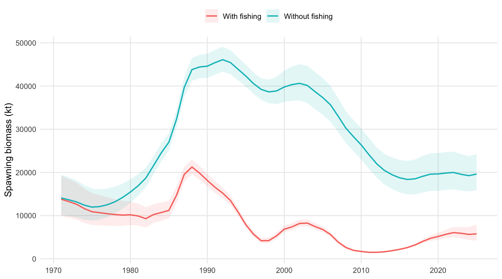
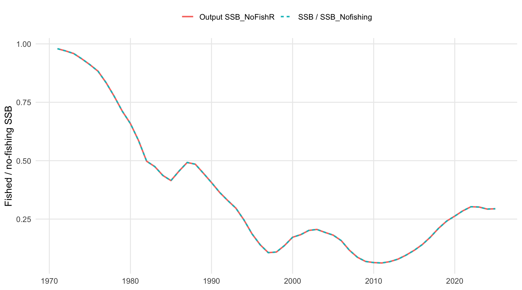
This report uses `r params$model_name`, stock `r params$stock`. The no-fishing spawning biomass is taken from `df1` in the model output object as `SSB_Nofishing`; the reported depletion comparison is taken from `SSB_NoFishR`, with `SSB0_Dynamic` included as a consistency check.

## Spawning Biomass

```{r}
#| label: fig-ssb-fished-unfished
#| fig-cap: "Estimated spawning biomass with fishing and the model counterfactual spawning biomass without fishing."
#| echo: false

biomass_series |>
  filter(metric == "Spawning biomass") |>
  ggplot(aes(year, estimate, color = scenario, fill = scenario)) +
  geom_ribbon(aes(ymin = lower, ymax = upper), alpha = 0.12, linewidth = 0) +
  geom_line(linewidth = 0.8) +
  labs(x = NULL, y = "Spawning biomass (kt)", color = NULL, fill = NULL) +
  theme_report()
```

```{r}
#| label: fig-ssb-bmsy-productivity
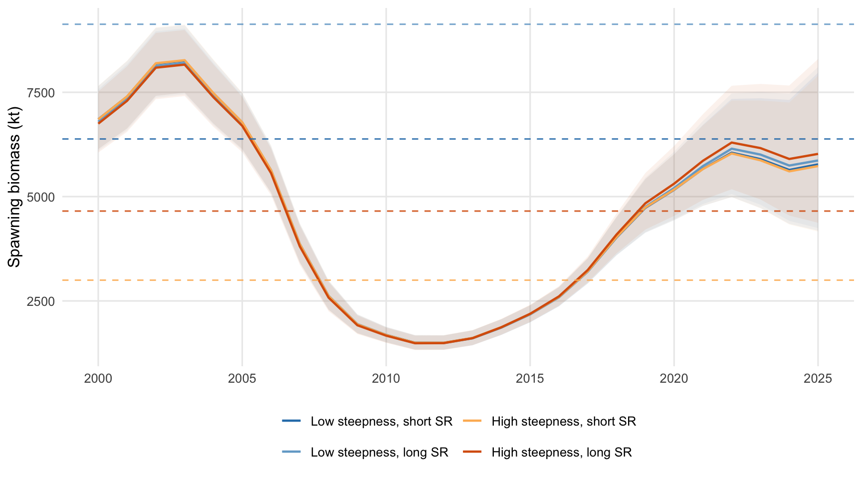
#| fig-cap: "Fished spawning biomass since 2000 across productivity assumptions. Dashed horizontal lines show Bmsy for each run."
#| echo: false

productivity_ssb_series |>
  filter(year >= 2000) |>
  ggplot(aes(year, estimate, color = scenario, fill = scenario)) +
  geom_ribbon(aes(ymin = lower, ymax = upper), alpha = 0.08, linewidth = 0, show.legend = FALSE) +
  geom_line(linewidth = 0.8) +
  geom_hline(
    data = bmsy_reference,
    aes(yintercept = Bmsy, color = scenario),
    inherit.aes = FALSE,
    linetype = "dashed",
    linewidth = 0.55,
    alpha = 0.85
  ) +
  scale_color_manual(values = productivity_scenario_colors) +
  scale_fill_manual(values = productivity_scenario_colors) +
  scale_x_continuous(breaks = seq(2000, max(productivity_ssb_series$year), by = 5)) +
  labs(x = NULL, y = "Spawning biomass (kt)", color = NULL, fill = NULL) +
  guides(
    fill = "none",
    color = guide_legend(nrow = 2)
  ) +
  theme_report() +
  theme(
    legend.position = "bottom",
    legend.box = "vertical"
  )
```

The post-2000 view in @fig-ssb-bmsy-productivity shows that the recent fished SSB trajectories are broadly similar, but the Bmsy reference levels diverge strongly among productivity assumptions. The low-steepness, long-SR run has the highest Bmsy (`r round(max(bmsy_reference$Bmsy, na.rm = TRUE), 0)` kt), while the high-steepness, short-SR run has the lowest Bmsy (`r round(min(bmsy_reference$Bmsy, na.rm = TRUE), 0)` kt). As a result, terminal status relative to Bmsy is mostly a productivity-assumption result: the same recent biomass scale is below the low-steepness Bmsy levels but above the high-steepness Bmsy levels.

```{r}
#| label: fig-ssb-difference-depletion
#| fig-cap: "Spawning biomass depletion ratio estimated as fished spawning biomass divided by no-fishing spawning biomass, compared with the reported depletion estimate."
#| echo: false

ssb_comparison |>
  filter(panel == "Depletion ratio") |>
  ggplot(aes(year, value, color = source, linetype = source)) +
  geom_line(linewidth = 0.85) +
  labs(x = NULL, y = "Fished / no-fishing SSB", color = NULL, linetype = NULL) +
  theme_report()
```

```{r}
#| label: tbl-ssb-terminal
#| tbl-cap: "Terminal-year spawning biomass impact and depletion comparison."
#| echo: false

kable(ssb_summary, digits = 4)
```

## Majuro Plot

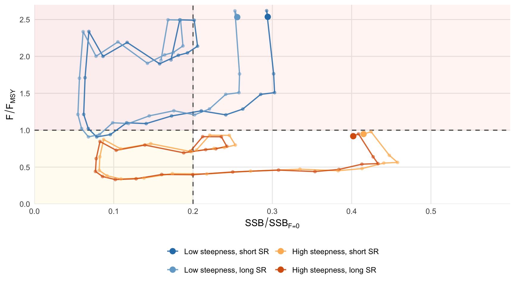
A Majuro plot is a WCPFC-style modification of a Kobe plot that puts fishing pressure on the y-axis as F/Fmsy, but puts biomass on the x-axis as depletion relative to unfished spawning biomass, SSB/SSB~F=0~, rather than SSB/Bmsy. The vertical line at 0.2 follows the common WCPFC tuna-stock display convention and is shown here only as a visual reference, not as a proposed jack mackerel limit reference point.

```{r}
#| label: fig-majuro-productivity
#| fig-cap: "Majuro plot for model 0.14 productivity assumptions, showing the 2000-2025 trajectory. Larger points mark terminal-year status. The vertical line marks SSB/SSB_F=0 = 0.2 for orientation and the horizontal line marks F/Fmsy = 1."
#| echo: false

majuro_series |>
  filter(year >= 2000) |>
  ggplot(aes(depletion, f_fmsy, color = scenario)) +
  annotate("rect", xmin = -Inf, xmax = 0.2, ymin = 1, ymax = Inf, fill = "#d73027", alpha = 0.08) +
  annotate("rect", xmin = 0.2, xmax = Inf, ymin = 1, ymax = Inf, fill = "#fc8d59", alpha = 0.08) +
  annotate("rect", xmin = -Inf, xmax = 0.2, ymin = -Inf, ymax = 1, fill = "#fee08b", alpha = 0.12) +
  geom_vline(xintercept = 0.2, linewidth = 0.65, linetype = "dashed", color = "gray35") +
  geom_hline(yintercept = 1, linewidth = 0.65, linetype = "dashed", color = "gray35") +
  geom_path(linewidth = 0.75, alpha = 0.85) +
  geom_point(aes(alpha = year == max(year)), size = 1.4, show.legend = FALSE) +
  geom_point(
    data = majuro_terminal,
    aes(depletion, f_fmsy, color = scenario),
    inherit.aes = FALSE,
    size = 3
  ) +
  scale_color_manual(values = productivity_scenario_colors) +
  scale_alpha_manual(values = c(`FALSE` = 0.45, `TRUE` = 1)) +
  coord_cartesian(xlim = c(0, majuro_x_upper), ylim = c(0, majuro_y_upper), expand = FALSE) +
  labs(x = expression(SSB / SSB[F == 0]), y = expression(F / F[MSY]), color = NULL) +
  guides(color = guide_legend(nrow = 2)) +
  theme_report() +
  theme(
    legend.position = "bottom",
    legend.box = "vertical"
  )
```

```{r}
#| label: tbl-majuro-terminal
#| tbl-cap: "Terminal-year Majuro plot coordinates for the productivity sensitivity runs."
#| echo: false

majuro_terminal |>
  transmute(
    model,
    scenario = as.character(scenario),
    year,
    SSB_over_SSB_F0 = depletion,
    F_over_Fmsy = f_fmsy
  ) |>
  kable(digits = 4)
```

In @fig-majuro-productivity, the low-steepness runs are above F/Fmsy = 1 in the terminal year, while the high-steepness runs are just below 1. The biomass axis shows the same productivity contrast: terminal SSB/SSB~F=0~ is lower for the low-steepness runs (`r paste(round(range(majuro_terminal$depletion[productivity_reference$steepness[match(majuro_terminal$model, productivity_reference$model)] == 0.65], na.rm = TRUE), 3), collapse = "-")`) than for the high-steepness runs (`r paste(round(range(majuro_terminal$depletion[productivity_reference$steepness[match(majuro_terminal$model, productivity_reference$model)] == 0.85], na.rm = TRUE), 3), collapse = "-")`). This is the same pattern as the Fmsy and Bmsy diagnostics: the stock-status interpretation is sensitive to the productivity assumption, even though the recent fished biomass trajectories are similar.

## Productivity Range

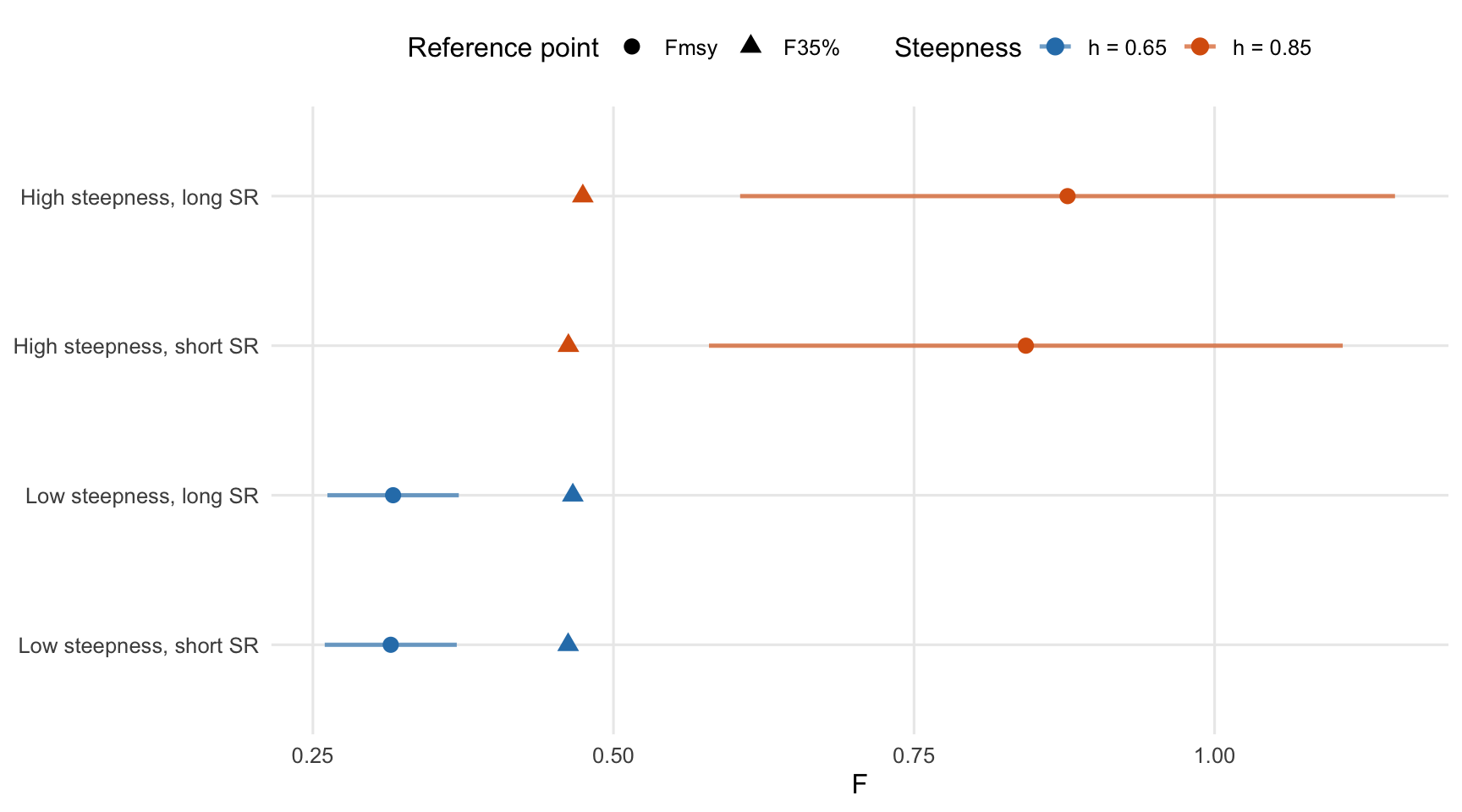
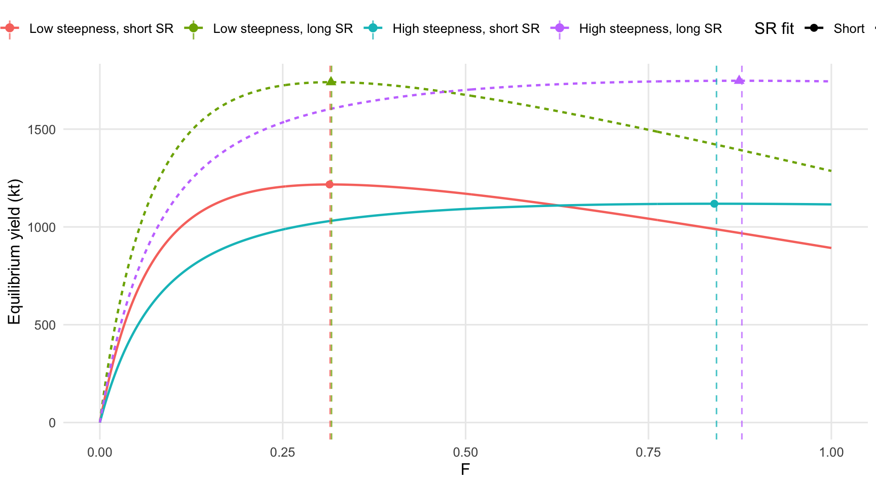
The productivity sensitivity runs span Fmsy values from `r round(min(productivity_reference$Fmsy, na.rm = TRUE), 3)` to `r round(max(productivity_reference$Fmsy, na.rm = TRUE), 3)`. The low-steepness runs produce the lower end of the range, while the high-steepness runs shift the F profile peak to substantially higher F values.

```{r}
#| label: tbl-productivity-reference
#| tbl-cap: "Fmsy values across productivity assumptions. Intervals use the reported standard errors from the .std files; profile_Fmsy is the F value at maximum yield in Fprof.yld."
#| echo: false

productivity_reference |>
  transmute(
    model,
    scenario = as.character(scenario),
    steepness,
    sr_years,
    Fmsy,
    Fmsy_se,
    F35_est,
    F_at_SPR35_profile,
    Fcur_Fmsy,
    Bmsy,
    Bmsy_se,
    Bcur_Bmsy,
    profile_Fmsy,
    MSY,
    SPR_at_profile_Fmsy
  ) |>
  kable(digits = 4)
```

```{r}
#| label: fig-productivity-fmsy-range
#| fig-cap: "Fmsy and F35% estimates across productivity assumptions. Horizontal bars show approximate 95% intervals for Fmsy using the reported standard errors."
#| echo: false

ggplot(productivity_reference, aes(Fmsy, scenario, color = steepness_label)) +
  geom_segment(
    aes(x = Fmsy_lower, xend = Fmsy_upper, y = scenario, yend = scenario),
    linewidth = 0.9,
    alpha = 0.65
  ) +
  geom_point(
    data = productivity_f_reference_points,
    aes(f, scenario, color = steepness_label, shape = reference),
    inherit.aes = FALSE,
    size = 3
  ) +
  scale_color_manual(values = c("h = 0.65" = "#2c7fb8", "h = 0.85" = "#d95f0e")) +
  scale_shape_manual(values = c("Fmsy" = 16, "F35%" = 17)) +
  labs(x = "F", y = NULL, color = "Steepness", shape = "Reference point") +
  theme_report()
```

The contrast in @fig-productivity-fmsy-range is mostly a steepness effect. The low-steepness cases put Fmsy near `r round(min(productivity_reference$Fmsy[productivity_reference$steepness == 0.65], na.rm = TRUE), 3)`-`r round(max(productivity_reference$Fmsy[productivity_reference$steepness == 0.65], na.rm = TRUE), 3)`, while the high-steepness cases shift Fmsy upward to `r round(min(productivity_reference$Fmsy[productivity_reference$steepness == 0.85], na.rm = TRUE), 3)`-`r round(max(productivity_reference$Fmsy[productivity_reference$steepness == 0.85], na.rm = TRUE), 3)`. Changing from the short to the long stock-recruit fitting period has a much smaller effect within each steepness assumption than changing steepness itself.

F35% is comparatively stable across these runs, ranging from `r round(min(productivity_reference$F35_est, na.rm = TRUE), 3)` to `r round(max(productivity_reference$F35_est, na.rm = TRUE), 3)`. That is expected because the SPR-based reference point is controlled mainly by selectivity, maturity, growth, and natural mortality, whereas Fmsy also depends strongly on the assumed stock-recruit productivity. Under low steepness, F35% sits above Fmsy, so it would imply a more aggressive F than the production-based MSY estimate. Under high steepness, Fmsy is well above F35%, so F35% becomes the more conservative reference point.

```{r}
#| label: fig-productivity-yield-profiles
#| fig-cap: "Yield profiles across productivity assumptions. Points mark the profile maximum and dashed vertical lines mark the reported Fmsy values."
#| echo: false

ggplot(productivity_yield_profiles, aes(f, yield, color = scenario, linetype = sr_fit)) +
  geom_line(linewidth = 0.8) +
  geom_vline(
    data = productivity_reference,
    aes(xintercept = Fmsy, color = scenario),
    inherit.aes = FALSE,
    linetype = "dashed",
    linewidth = 0.55,
    alpha = 0.75
  ) +
  geom_point(
    data = productivity_reference,
    aes(profile_Fmsy, MSY, color = scenario, shape = sr_fit),
    inherit.aes = FALSE,
    size = 2.4
  ) +
  labs(x = "F", y = "Equilibrium yield (kt)", color = NULL, linetype = "SR fit", shape = "SR fit") +
  theme_report()
```

## SPR Reference Point

```{r}
#| label: tbl-spr-reference
#| tbl-cap: "SPR reference point from the refreshed model run. SBF35 is interpolated from the yield profile at SPR = 0.35."
#| echo: false

kable(spr_reference, digits = 4)
```

```{r}
#| label: fig-f-profile
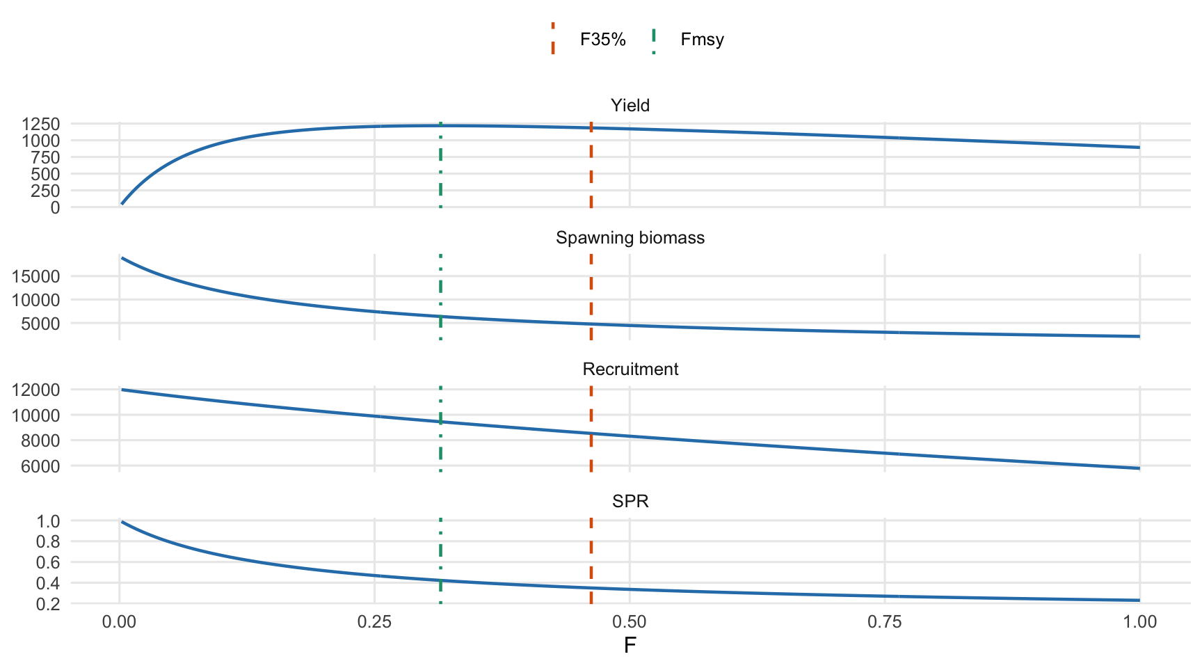
#| fig-cap: "F profile from Fprof.yld. Vertical lines mark F35% and Fmsy on the profile."
#| echo: false

ggplot(f_profile, aes(f, value)) +
  geom_line(linewidth = 0.8, color = "#2c7fb8") +
  geom_vline(
    data = f_reference_lines,
    aes(xintercept = f, color = reference, linetype = reference),
    linewidth = 0.8
  ) +
  facet_wrap(~quantity, scales = "free_y", ncol = 1) +
  scale_color_manual(values = c("F35%" = "#d95f0e", "Fmsy" = "#1b9e77")) +
  scale_linetype_manual(values = c("F35%" = "dashed", "Fmsy" = "dotdash")) +
  labs(x = "F", y = NULL, color = NULL, linetype = NULL) +
  theme_report()
```

```{r}
#| label: tbl-f-ratio-by-fishery
#| tbl-cap: "Fishery ratios used to apportion F-based reference points. Ratios are based on mean end-year F by fishery, matching the Fratio calculation used for SPR rates."
#| echo: false

kable(fishery_f_ratio, digits = 4)
```

## Total Biomass

```{r}
#| label: fig-total-fished-unfished
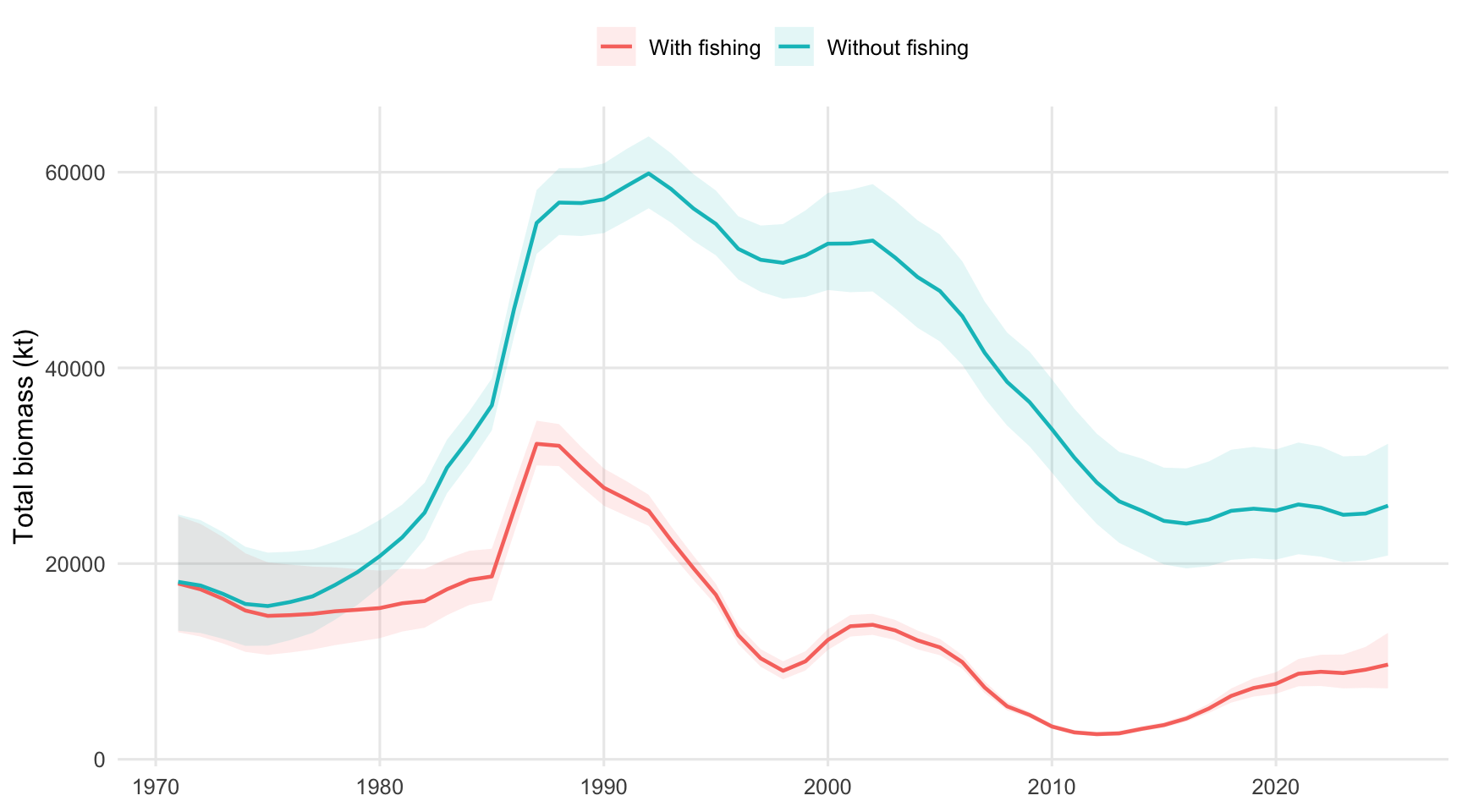
#| fig-cap: "Estimated total biomass with fishing and the model counterfactual total biomass without fishing."
#| echo: false

biomass_series |>
  filter(metric == "Total biomass") |>
  ggplot(aes(year, estimate, color = scenario, fill = scenario)) +
  geom_ribbon(aes(ymin = lower, ymax = upper), alpha = 0.12, linewidth = 0) +
  geom_line(linewidth = 0.8) +
  labs(x = NULL, y = "Total biomass (kt)", color = NULL, fill = NULL) +
  theme_report()
```

```{r}
#| label: fig-total-difference-ratio
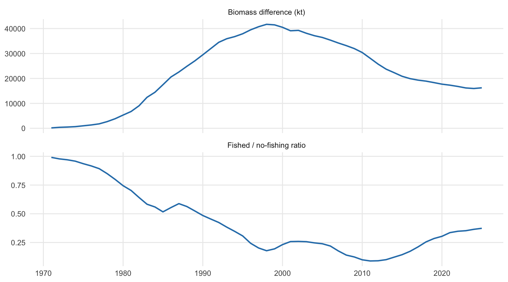
#| fig-cap: "Absolute difference between no-fishing and fished total biomass compared with the total-biomass ratio."
#| echo: false

biomass_wide |>
  filter(metric == "Total biomass") |>
  transmute(
    year,
    `Biomass difference (kt)` = difference,
    `Fished / no-fishing ratio` = ratio
  ) |>
  pivot_longer(-year, names_to = "panel", values_to = "value") |>
  mutate(panel = factor(panel, levels = c("Biomass difference (kt)", "Fished / no-fishing ratio"))) |>
  ggplot(aes(year, value)) +
  geom_line(linewidth = 0.85, color = "#2c7fb8") +
  facet_wrap(~panel, scales = "free_y", ncol = 1) +
  labs(x = NULL, y = NULL) +
  theme_report()
```

```{r}
#| label: tbl-total-terminal
#| tbl-cap: "Terminal-year total biomass impact and fished/no-fishing ratio."
#| echo: false

kable(total_summary, digits = 4)
```