Jack mackerel base model: MCMC uncertainty

What the run shows

The default ADNUTS run sampled 1,593 active parameters in the single-stock base model h1_1.06. Three chains each completed 2,000 iterations; the first 1,000 iterations of each chain were warmup. The summaries below use the remaining 3,000 draws.

The default run needs further sampling checks

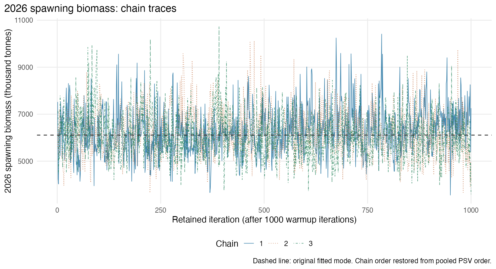
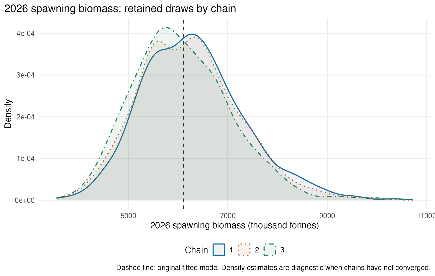
The run completed with zero retained divergences and zero tree-depth-limit events. Some parameters have slow mixing and fail the screening criteria below. The figures and intervals provide an exploratory description of these retained draws. Further sampling and validation are needed before using these uncertainty estimates for management advice.

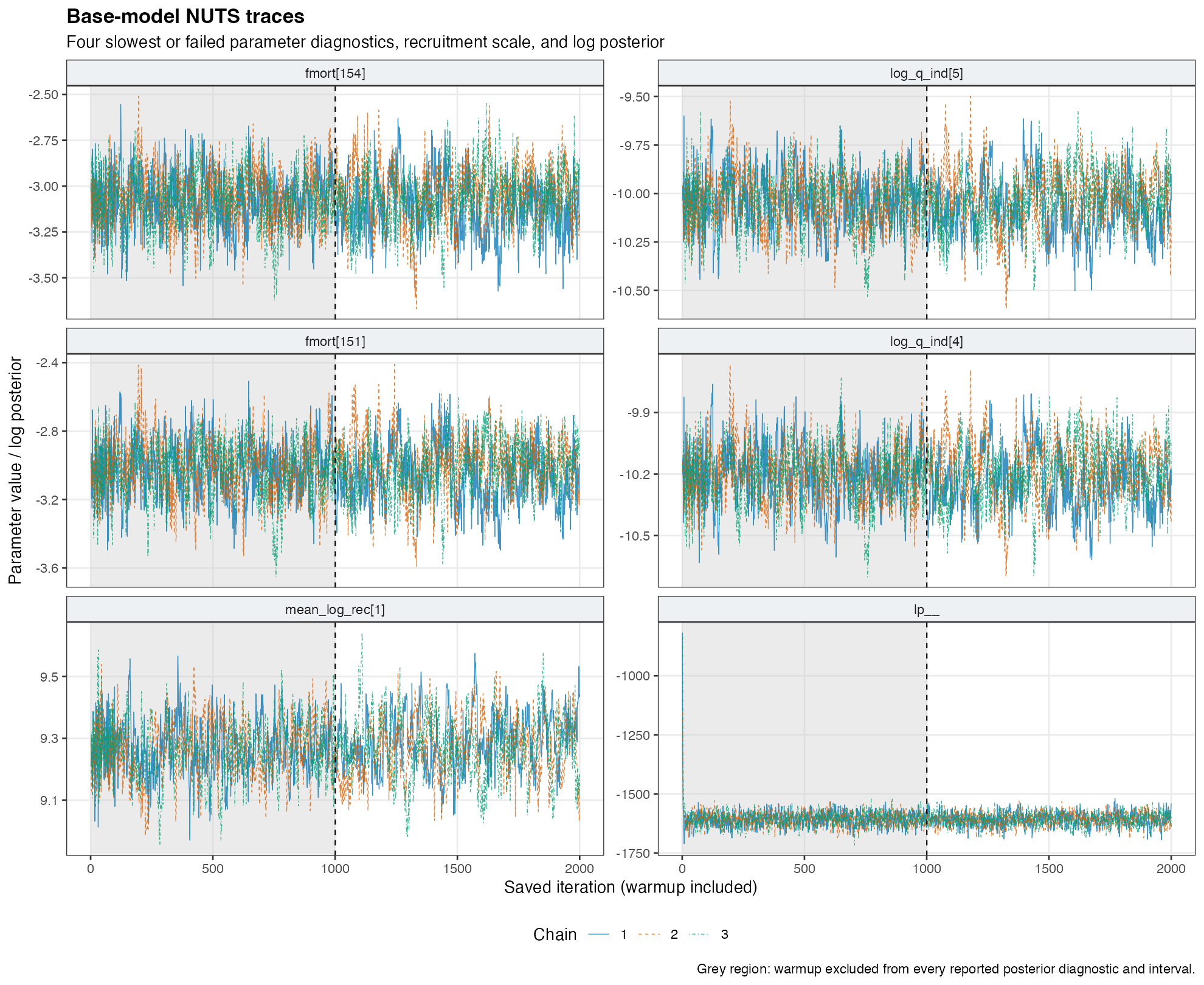
The largest finite parameter R-hat is 1.055. The smallest finite bulk and tail effective sample sizes are 83 and 150, respectively. There are 0 divergent transitions and 0 maximum-tree-depth events among 3,000 retained iterations.

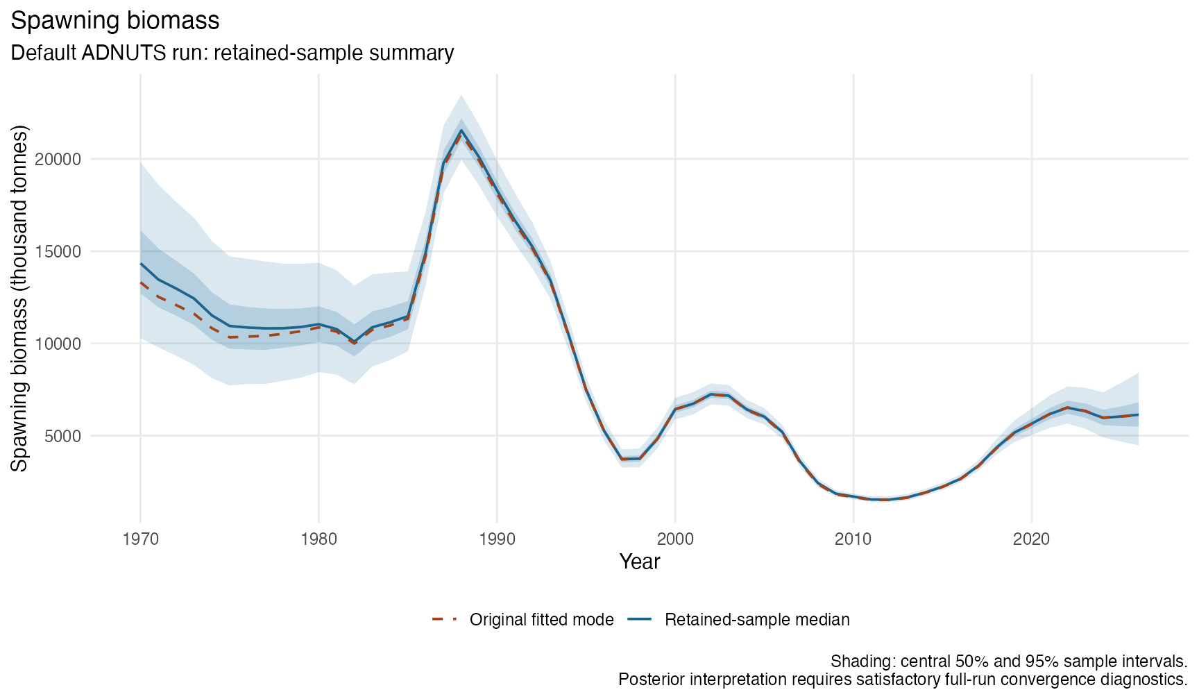
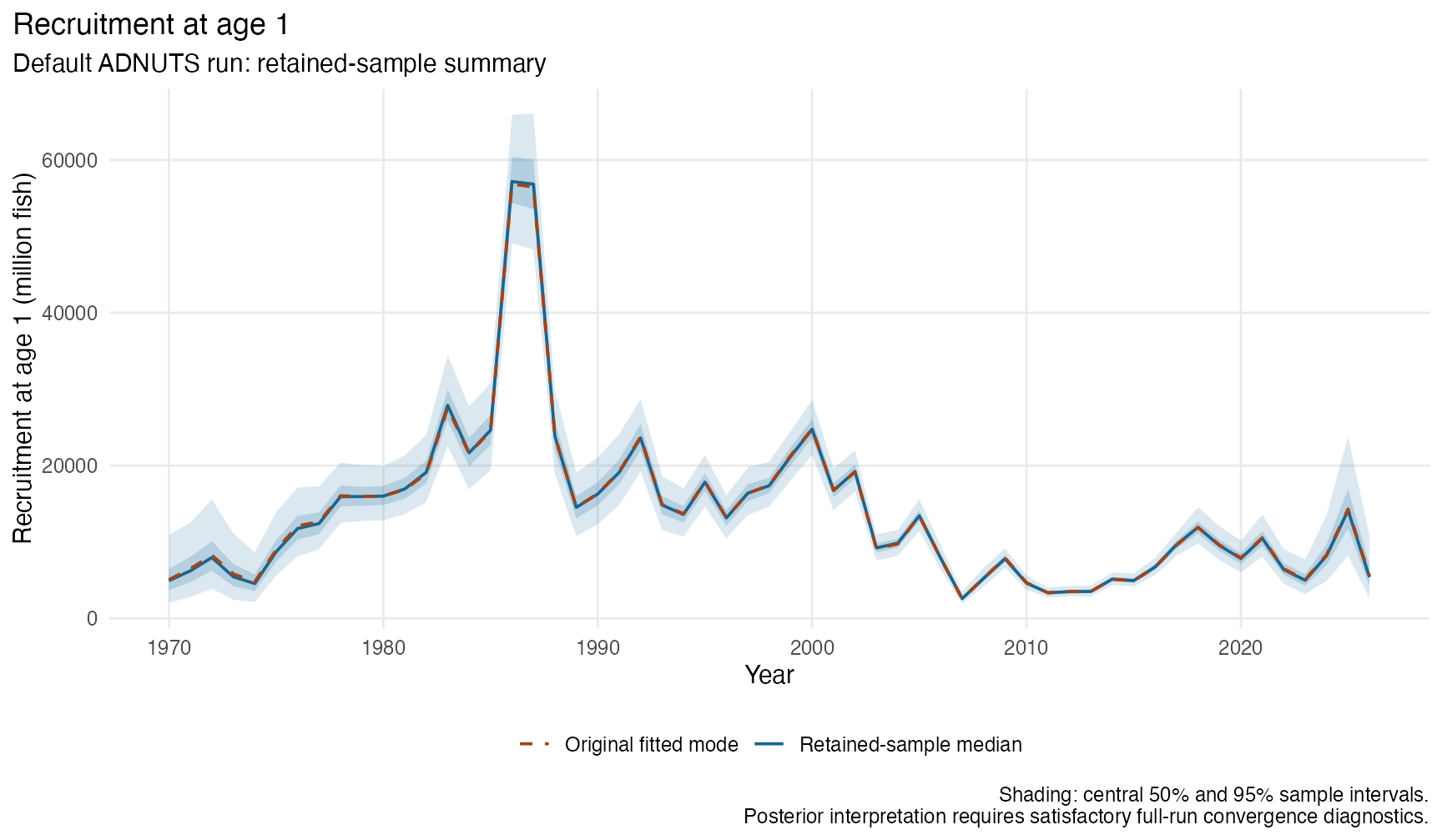
The 2026 spawning-biomass sample median is 6.14 million tonnes, with an exploratory central 95% interval of 4.47–8.43 million tonnes. Its R-hat is 1.018, so this quantity also needs further between-chain agreement checks. Recruitment at age 1 has a sample median of 5.38 billion fish; detailed units, intervals and diagnostics are given below.

This separate working document accompanies the assessment and provides an analysis for Scientific Committee review.

Model and sampler

The SC14 assessment source identifies model 1.06 as the final model in the working comparison. This run uses its single-stock hypothesis, with data from 1970 through 2026, control file h1_1.06.ctl, data file 1.06.dat, and the saved fitted parameter file. The run retains the working assessment’s 2026 catch projections and other model inputs. This analysis covers the single-stock hypothesis.

The fitted objective was 1384.75151390345. An isolated evaluation at the saved parameters reproduced it to within \(2\times10^{-9}\). The original fitted maximum gradient component was approximately 0.000167. The preparation evaluated the saved parameter values using zero optimization iterations. The original fitted gradient supplies the convergence evidence for that mode.

The target is proportional to the exponential of the negative complete ADMB objective over the active parameters and their existing bounds. Existing likelihoods, penalties and priors remain in place; ADMB applies the required Jacobian for its sampling transformations. Parameters fixed in the control file remain fixed, including natural mortality (0.28 per year), steepness (0.65), and recruitment deviation standard deviation (0.6). The run uses the existing prior specification.

ADNUTS provides NUTS sampling for ADMB models. The installed package’s sample_nuts() defaults were used directly.

Setting	Value
Model executable	ADMB 13.2, `jjm2`
R package	adnuts 1.1.2
Chains	3
Iterations per chain	2,000 total; 1,000 warmup; 1,000 retained
Total retained draws	3,000
Initial mass matrix	Unit diagonal
Mass matrix adaptation	Diagonal adaptation during warmup
Target acceptance probability	0.8
Maximum tree depth	12
Step size	Adapted
Thinning	1
Initialization	Package default: all chains start from the saved fitted mode
Chain seeds	4754034, 193486, 8644402
Sampling wall time	0.52 hours

The root R seed was 20260910; the package generated the individual chain seeds. Sampler controls retained their default values throughout this run. The -fut_sel 3 model argument preserves the assessment’s future-selectivity convention. Interpretation focuses on historical fitted quantities. Derived quantities were evaluated from retained draws after sampling, keeping the sampler’s default mceval = FALSE unchanged.

Do the chains agree?

R-hat measures agreement between chains, while effective sample size (ESS) accounts for autocorrelation. The screening used here requires rank-normalized split R-hat no greater than 1.01 and bulk and tail ESS of at least 400. The ESS threshold of 400 is the screening choice for this report. These checks follow the definitions in the Stan diagnostic guidance. Convergence assessment combines these numerical screens with chain plots and checks of model exploration. All chains start at the same mode under the requested defaults; suitably dispersed starts would provide an additional check of exploration across modes.

Table 1: Parameter checks across 1,593 active parameters. Log posterior is assessed separately. Failure counts overlap.

Check	Parameters
Pass all parameter screens	1227
R-hat > 1.01	220
Bulk ESS < 400	329
Tail ESS < 400	95
Undefined diagnostics	0
Nonfinite parameter draws	0
Constant parameter in any chain	0

Table 2: Sampler checks use only the 1,000 retained iterations in each chain.

Chain	Retained	E-BFMI	Mean acceptance	Mean leapfrog steps
1	1000	1.053	0.807	108
2	1000	1.037	0.812	117
3	1000	0.984	0.812	125

Divergences can signal biased exploration. Maximum-tree-depth events indicate that the sampler reached its trajectory-length limit. Energy Bayesian fraction of missing information (E-BFMI) is computed within each retained chain; values below 0.3 are flagged. The full screening requires zero divergences, zero depth-limit events, finite diagnostics, and E-BFMI of at least 0.3 in every chain.

Table 3: Ten parameters with the weakest between-chain agreement, followed by lowest bulk ESS. Native ADMB parameter scales are retained.

Parameter	R-hat	Bulk ESS	Tail ESS	MCSE of mean
fmort[154]	1.055	89	442	0.0168
log_q_ind[5]	1.053	119	406	0.0134
fmort[151]	1.052	126	504	0.0147
log_q_ind[4]	1.051	122	390	0.0129
fmort[153]	1.050	121	460	0.0149
fmort[152]	1.049	125	407	0.0153
fmort[144]	1.048	131	451	0.0191
fmort[149]	1.047	128	472	0.0161
fmort[147]	1.047	132	468	0.0163
fmort[145]	1.046	137	452	0.0175

Separate chain traces for selected model parameters and log posterior. A shaded region marks the first 1000 warmup iterations, which are excluded from all reported summaries. — Figure 1: Six parameter traces, including the weakest parameter diagnostics, recruitment scale and log posterior. Each chain is distinguished by color and line type; warmup is shaded.

Chain-specific density curves for six selected quantities using only retained draws. Different line types and colors identify the three chains. — Figure 2: Retained-draw marginal distributions for the same parameters, shown separately by chain. Agreement in these plots is assessed alongside the numerical diagnostics.

Biomass and recruitment uncertainty

These summaries use all 3,000 retained draws, with chain membership preserved for diagnostics. Intervals are the equal-tailed 2.5th and 97.5th percentiles. These intervals describe the sampled draws. Further sampling is needed to support reliable posterior credible intervals.

Table 4: 2026 summaries from all 3,000 retained draws. Intervals are exploratory because the full-model sampling checks fail.

Quantity	Units	Fitted mode	Sample median	2.5th–97.5th percentiles	R-hat	Bulk ESS	Tail ESS
Spawning biomass	thousand tonnes (kt)	6,109	6,136	4,474–8,425	1.018	557	1,631
Recruitment at age 1	million fish	5,560	5,383	2,605–10,768	1.000	2,638	2,098

The original fitted values are 6,108.87 thousand tonnes of spawning biomass and 5,559.86 million recruits at age 1 in 2026. The mode curves below were regenerated at the saved fitted parameters and checked against the original objective. The central 50% band shows the interquartile range; the wider band contains the central 95% of retained values.

The derived-quantity screen flags 39 of 114 quantity-year combinations (spawning biomass and recruitment over 1970–2026). Its maximum R-hat is 1.040, and minimum bulk/tail ESS are 144/253. Overall sampling assessment combines these derived-quantity diagnostics with the full set of parameter and sampler checks.

Historical spawning biomass in thousand tonnes, with sample median and shaded central 50 and 95 percent intervals. A dashed line marks the original fitted mode; the intervals are exploratory given incomplete chain agreement. — Figure 3: Spawning biomass over 1970–2026: retained-sample median, central 50% and 95% intervals, and the original fitted mode.

Age-one recruitment in million fish by year, with retained-sample median, central 50 and 95 percent intervals, and dashed fitted-mode estimates. — Figure 4: Recruitment at age 1 over 1970–2026: retained-sample median, central 50% and 95% intervals, and the original fitted mode.

2026 spawning biomass from each of the three chains across 1000 retained iterations, with a horizontal fitted-mode reference. Chain line styles and colors allow assessment of overlap and drift. — Figure 5: The three retained chains for 2026 spawning biomass. The horizontal reference is the original fitted mode.

Three separate density curves for retained 2026 spawning-biomass draws, with a fitted-mode vertical reference, allowing visual comparison of chain locations and spreads. — Figure 6: Chain-specific distributions for 2026 spawning biomass, using retained draws only.

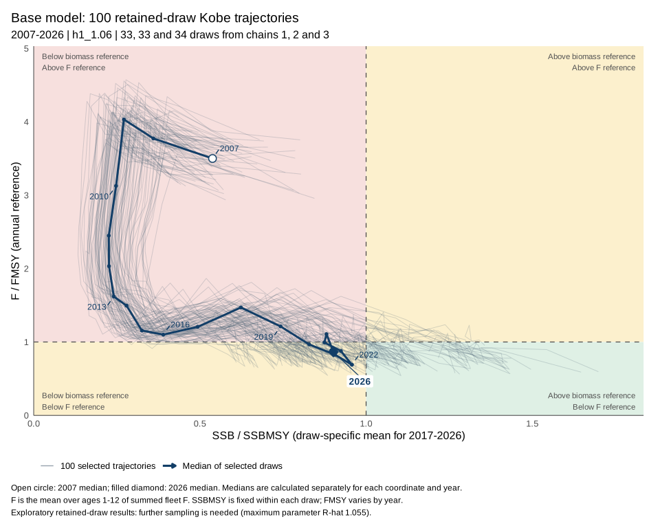
100 Kobe trajectories, 2007–2026

The Kobe display follows 100 retained draws through the last 20 model years, 2007–2026. Draws were sampled without replacement using seed 20260910: 33 from chain 1, 33 from chain 2 and 34 from chain 3. Each trajectory follows the same parameter draw across all 20 years. These are historical fitted trajectories conditional on the base model; the full-run mixing limitations also apply here.

Explore the interactive Kobe plot to select a trajectory and inspect its year-specific values. Download compact Kobe-format data (iter, year, stock, harvest) or all quantities and draw identities. Each CSV has 2,000 rows: 100 draws × 20 years.

The horizontal coordinate is spawning biomass divided by the draw’s mean annual MSY spawning biomass over 2017–2026, following the assessment’s fixed-biomass-reference convention. The vertical coordinate is fishing mortality divided by the matching annual FMSY. Fishing mortality is the unweighted mean across all 12 model ages after summing the four fleets:

\[ \mathrm{stock}_{d,y}=\frac{SSB_{d,y}}{\operatorname{mean}_{t=2017}^{2026}(SSBMSY_{d,t})}, \qquad \mathrm{harvest}_{d,y}=\frac{\frac{1}{12}\sum_{f=1}^{4}\sum_{a=1}^{12}F_{d,f,y,a}}{FMSY_{d,y}}. \]

Both coordinates are dimensionless. Reference lines at one mark each denominator. The thick curve joins the coordinate-wise medians of the 100 selected draws for each year; each coordinate is summarized separately to provide a visual guide to the selected draws.

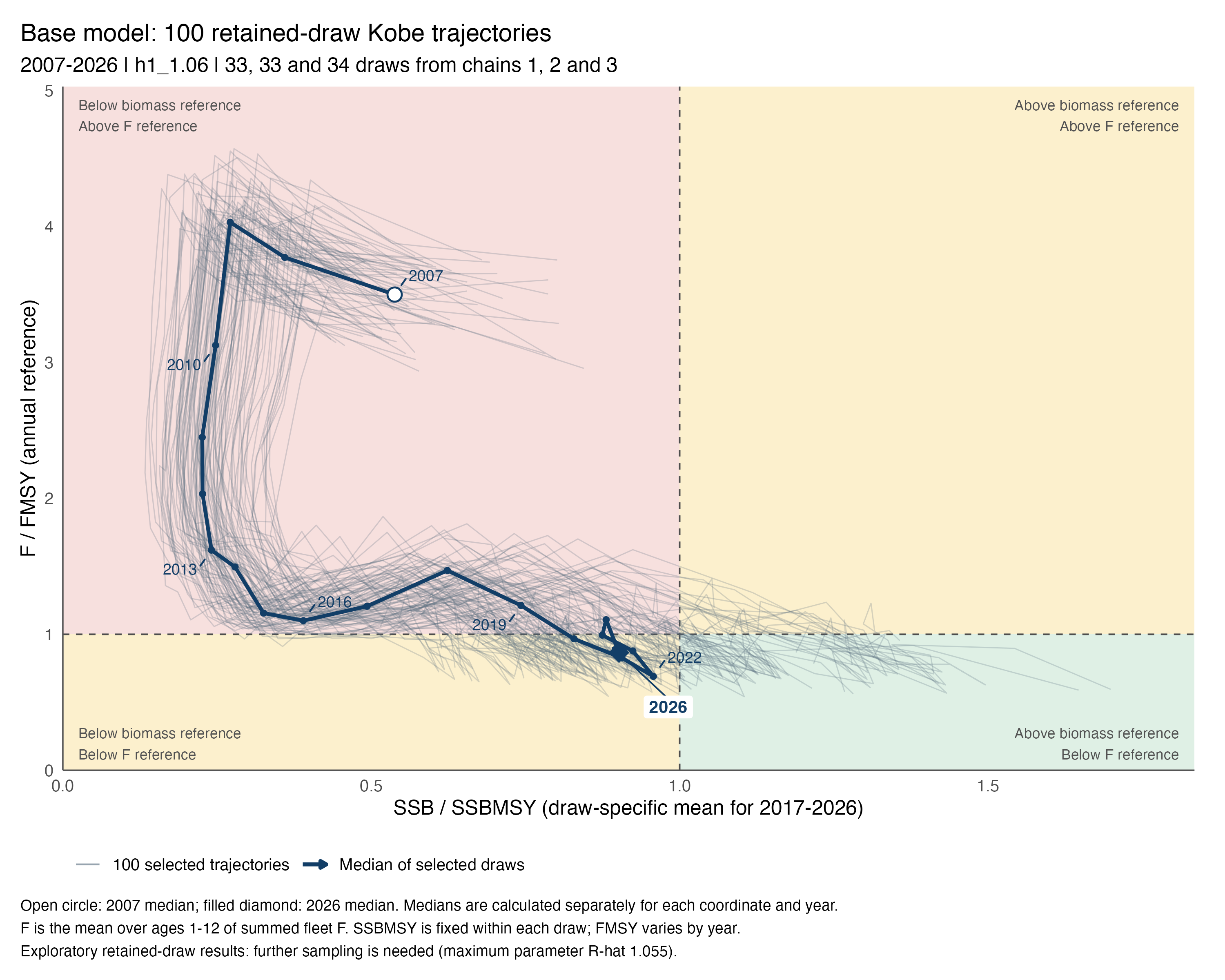
Kobe plot of 100 retained posterior trajectories over 2007 to 2026. Horizontal axis is spawning biomass relative to each draw's mean 2017 to 2026 MSY biomass; vertical axis is fishing mortality relative to annual FMSY. The median moves from approximately 0.54 and 3.50 in 2007 to 0.90 and 0.86 in 2026. Reference lines divide the plane at one; these are exploratory results because full-run chain screening failed. — Figure 7: One hundred matched Kobe trajectories for 2007–2026. Thin lines show selected draws; the thick line joins their annual coordinate-wise medians. The open circle marks 2007 and the filled diamond marks 2026.

Annual reference points come from the frozen model’s existing annual MSY routine. The original evaluation omitted annual FMSY, so a reporting-only copy emitted that quantity and the native F/FMSY check for the selected draws. The added output leaves their spawning biomass, fishing mortality and annual MSY biomass identical to the original evaluation. All annual reference points are positive and none reaches the routine’s fishing-mortality grid limits. See the Kobe methods and data dictionary, selection manifest, validation record, and supplementary reproduction files.

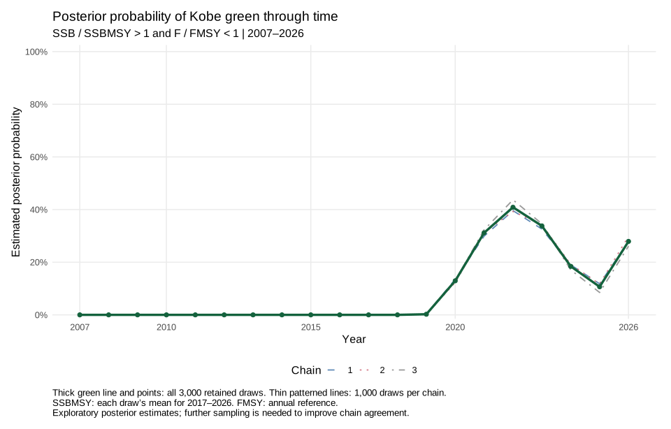
Probability of Kobe green through time

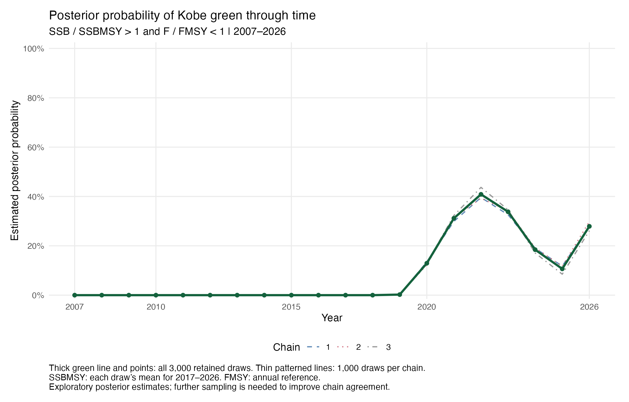
For each year from 2007 through 2026, the estimated posterior probability of being in the green quadrant is the proportion of all 3,000 retained draws with spawning biomass above its MSY reference and fishing mortality below FMSY:

\[ \widehat{P}(\mathrm{green}_y\mid\mathrm{data},\mathrm{model})= \frac{1}{3000}\sum_{d=1}^{3000} \mathbf{1}\!\left[\mathrm{stock}_{d,y}>1\;\text{and}\;\mathrm{harvest}_{d,y}<1\right]. \]

The two conditions are evaluated jointly within each draw, preserving their posterior dependence. The reference definitions match the Kobe trajectories above: each draw’s mean SSBMSY for 2017–2026 and annual FMSY. Both inequalities are strict. Each chain contributes 1,000 retained draws, giving equal chain weights.

The 2026 estimate is 27.9%, corresponding to 837 of 3,000 draws in green. These are exploratory posterior estimates conditional on this base model. Further sampling is needed to improve the full model’s chain agreement and strengthen the probability estimates.

Annual estimated posterior probability of simultaneously exceeding the MSY spawning-biomass reference and having fishing mortality below annual FMSY over 2007 to 2026. A thick green line shows the proportion across all 3000 retained draws, and three patterned lines show individual-chain proportions. The downloadable table gives every annual value and Monte Carlo precision estimate. — Figure 8: Estimated posterior probability of the Kobe green quadrant for each year, using all 3,000 retained draws. The thick green line and points give the pooled estimate; thin patterned lines give estimates from each chain.

Table 5: Annual estimated posterior probabilities of Kobe green. Each year uses 3,000 retained draws. Monte Carlo standard errors (MCSE) are expressed in percentage points.

Year	Green draws	Probability (%)	Chain range (%)	MCSE (percentage points)
2007	0	0.0	0.0–0.0	—
2008	0	0.0	0.0–0.0	—
2009	0	0.0	0.0–0.0	—
2010	0	0.0	0.0–0.0	—
2011	0	0.0	0.0–0.0	—
2012	0	0.0	0.0–0.0	—
2013	0	0.0	0.0–0.0	—
2014	0	0.0	0.0–0.0	—
2015	0	0.0	0.0–0.0	—
2016	0	0.0	0.0–0.0	—
2017	0	0.0	0.0–0.0	—
2018	0	0.0	0.0–0.0	—
2019	7	0.2	0.2–0.3	0.1
2020	388	12.9	12.3–13.5	0.7
2021	935	31.2	29.9–32.3	0.9
2022	1226	40.9	39.3–43.7	1.0
2023	1014	33.8	32.6–34.6	0.9
2024	553	18.4	17.1–19.2	1.0
2025	320	10.7	8.5–11.8	0.9
2026	837	27.9	26.1–29.8	1.1

MCSE measures Monte Carlo precision of the estimated probability while accounting for correlation within chains. The calculation uses the binary green-quadrant indicator and preserves chain identity. The chain range shows the smallest and largest of the three chain-specific estimates. For years with a constant indicator across retained draws, the table reports the observed proportion and marks MCSE with a dash. A zero count describes the finite set of sampled draws. The full-model diagnostics above provide the context for interpreting these probabilities.

Download the annual probability table, chain-specific estimates, all draw-level coordinates and green indicators, or vector figure. The calculation and evaluation scripts and validation record document the derivation. The previously displayed 100 trajectories retain their original draw selection; the probability calculation uses the full retained sample.

Interpretation and next steps

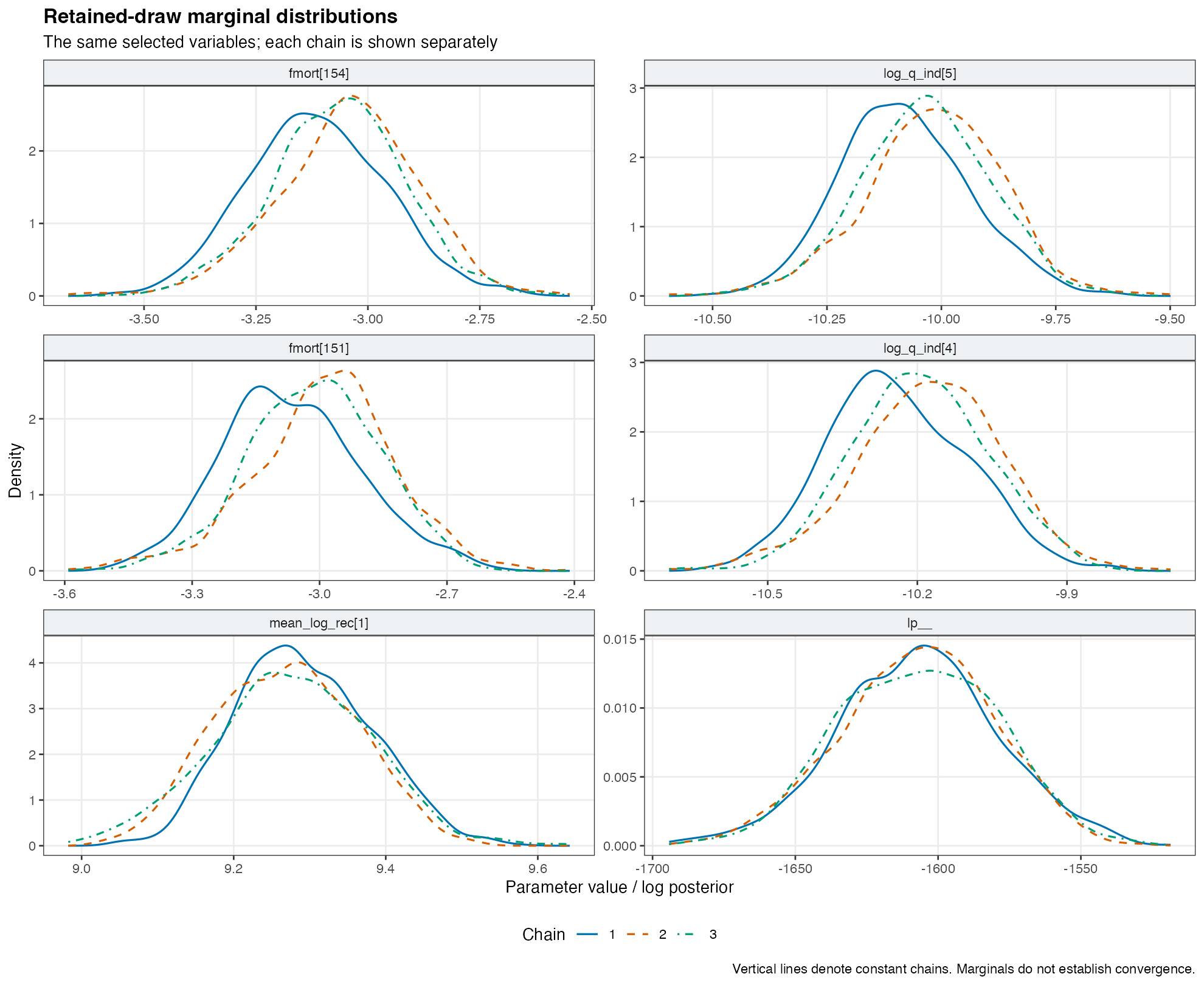
The chain-specific marginal plots show a shift in chain 1 for several of the slowest fishing-mortality and survey-catchability parameters. This agrees with the elevated R-hat and low ESS. Increasing the retained run length and checking suitably dispersed starting points are reasonable next checks; either would be a separately labelled follow-up run. The current analysis preserves the requested defaults.

What uncertainty is covered?

MCMC explores parameter uncertainty conditional on this single-stock model. Alternative stock hypotheses, additional processes, different data treatments and fixed parameter choices can be assessed through separate sensitivity analyses. The defaults initialize every chain at the same mode. A run that needs further work should be followed by a separately labelled analysis with justified changes to initialization, run length or sampler controls.

The Kobe calculation constructs stock-wide fishing mortality from F at age across all four fleets. The model’s native Fbar field describes a fishery-specific parameter, and its depletion fields describe total-biomass ratios. The source notes record these definitions so each reported quantity retains its biological meaning.

Files and reproducibility

Editable Quarto source
Recorded run settings and sampling diagnostic summary
All parameter summaries and chain diagnostics
Derived quantity summaries and source notes
Kobe data in R format, vector figure, and trajectory extraction script
Software environment and source/output checksums
Reproduction instructions and reproducibility files, including the exact model source, control, data, saved parameter input, and analysis scripts

The raw fit and full ADMB evaluation output are retained in the local run archive. Their checksums identify the draws used here. Report rendering uses the saved summaries and figures from the completed run.

Validation record

Check	Outcome	Evidence
Base-model identity and inputs	Pass	Frozen file hashes; original and prepared objective agree within 2 × 10⁻⁹
Requested sampler defaults	Pass	Recorded package formals, resolved controls and all three executed commands
Sampling completion and draw order	Pass	2,000 × 3 iterations; all 4,779,000 pooled parameter values match the retained fit bit for bit
Numerical sampler diagnostics	Pass	Zero retained divergences and zero depth-limit events; E-BFMI ≥0.984
Parameter mixing and precision	Fail	366/1,593 active parameters fail one or more reported screens
Native derived-output completeness	Pass	All 3,000 draws and 57 years verified; all 20 native output types inventoried
Kobe draw selection and coordinates	Pass	100 distinct retained draws; 20 years each; unchanged native quantities and matching annual reference points
Annual Kobe green probability	Pass	All 3,000 retained draws and 20 years; joint event counts, chain weights and original 100-draw coordinates verified
Reported results	Pass	Tables and figures read the saved, checked CSVs; independent parameter diagnostic calculation agrees
HTML, navigation, figure descriptions and file links	Pass	Rendered artifact, figure review and scoped local-link validation recorded in the release checks
Manual screen-reader review	Pending	A manual review remains an additional validation step

These checks document the numerical, file and visual validation completed for this analysis.