SCW17/Paper-03: Management procedures inventory for jack mackerel MSE
Inventory of jmMSE MP definitions, modules, source scripts, and exploratory variants

SPRFMO
1 Document Status and Traceability
This paper is an SCW17-branded copy of the local jmMSE management-procedure inventory. It is intended to make the management procedure (MP) definitions easier to review in the SCW17 documentation set without recreating or altering the scientific analyses in jmMSE.
| Item | Description |
|---|---|
| SCW17 identifier | SCW17/Paper-03 |
| SCW17 source file | doc/SCW17-Paper-03-Management-Procedures-Inventory.qmd |
| Source repository | /Users/jim/_mymods/sprfmo/jmMSE |
| Source file | management_procedures_inventory.qmd |
| Source branch and commit at sync | devel, bbb7f83 |
| Sync date | 2026-06-07 |
| Source file Git status at sync | Local untracked file in jmMSE |
| SCW17 role | Technical inventory supporting candidate MP discussion and documentation |
No benchmark results, operating-model assumptions, management-procedure definitions, performance metric definitions, or reference points are changed by this transfer. The inventory below preserves the source descriptions and differentiates between MP material found in tracked jmMSE files and MP material found in local exploratory files.
2 Purpose
This document inventories the management procedures (MPs) currently represented in the jmMSE checkout for SPRFMO jack mackerel MSE work. It is intended as a technical orientation document, not as a replacement for the formal working papers or the executable model scripts.
The repository does not currently contain one formal MP registry. Instead, MPs are specified inline as mpCtrl() objects in scripts and exploratory notebooks. Each mpCtrl() generally combines:
- an estimator or empirical status module, stored in the
estcomponent; - a harvest control rule, stored in the
hcrcomponent; - an implementation system, stored in the
isyscomponent.
In simple terms, the MP answers these questions:
- What information does the management procedure observe or estimate?
- How does that information get translated into a recommended catch or effort?
- How is the recommendation allocated or implemented across fleets/stocks?
- How is the procedure tuned and evaluated against performance metrics?
No scientific assumptions are changed by this document. It only describes MP definitions already present in the checkout.
3 Source Status
The inventory below distinguishes between two kinds of sources.
| Source class | Meaning | Files |
|---|---|---|
| Tracked repository files | Files committed to the current Git repository history. These are the most defensible sources for saying what is included in the repository. | demo.R, model_shortcut.R, model_fixed.R, model_spict.R, model_explore.R, report_JM-WP-MSE-01_Candidate_Management_Procedures_for_Jack_Mackerel.Rmd |
| Local exploratory files | Files present in the working tree but currently untracked by Git. They are very useful for understanding active MP development, but they are not yet part of repository history unless added and committed. | MP_cases_Jim.R, MP_test_Jim.R, jim_demo.R, SPRFMO_jack_mackerel_alternative.qmd, mpCtrl_mseCtrl_summary.qmd, buffer.hcr.qmd, bufferdelta_hcr_plot.qmd |
That distinction matters. For formal documentation, the tracked scripts provide the minimum confirmed MP set. The untracked scripts expand the practical working inventory substantially, especially for CPUE z-score, TAC-change, banking/borrowing, and multi-index MP variants.
4 MP Architecture
The MSE code uses the mse package style of MP composition. An MP is typically constructed as an mpCtrl() object whose components are mseCtrl() objects. The pattern is:
ctrl <- mpCtrl(list(
  est  = mseCtrl(method = some_estimator, args = list(...)),
  hcr  = mseCtrl(method = some_hcr,       args = list(...)),
  isys = mseCtrl(method = some_isys,      args = list(...))
))
4.1 Flow
The MP flow is shown in Figure 1. The upper lane describes the information available to the MP. The lower lane describes the decision rule, implementation system, projected MSE run, and tuning feedback.
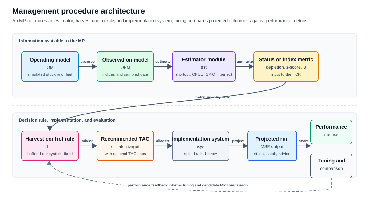
jmMSE.
4.2 Components
The component vocabulary in this checkout is:
| Component | Role | Examples in this checkout |
|---|---|---|
est |
Produces the information used by the HCR. This may be a perfect observation of the OM, a shortcut assessment, a CPUE/index metric, a z-score, a SPiCT fit, or a meta-estimator combining multiple indices/stocks. | perfect.sa, shortcut.sa, cpue.ind, cpuescore.ind, cpuescore2.ind, cpuescores.ind, balanced_cpuescore.ind, meta.est, spict.sa |
hcr |
Converts estimated status or index information into a catch recommendation or multiplier. | fixedC.hcr, hockeystick.hcr, buffer.hcr, bufferdelta.hcr, bufferdelta2.hcr, meta.hcr |
isys |
Converts the HCR output into implemented catch by fishery/stock, often using recent catch shares. | split.is, bank_borrow.is |
| tuning | Searches over HCR parameters to hit a target performance probability, usually a probability of Kobe green. | tunebisect(), mps(), FLmses() |
| performance | Scores MP runs against output statistics. | performance(), writePerformance(), periodsPerformance() |
5 Summary Inventory
| MP family | Status | Estimator/status module | HCR | Implementation | Main source files |
|---|---|---|---|---|---|
| Fixed catch reference MP | Tracked | perfect.sa |
fixedC.hcr |
split.is |
model_fixed.R |
| Shortcut depletion plus hockeystick HCR | Tracked | shortcut.sa on depletion |
hockeystick.hcr |
split.is |
demo.R, model_shortcut.R |
| Empirical CPUE/index plus buffer HCR | Tracked | cpue.ind |
buffer.hcr |
split.is |
demo.R, model_explore.R |
| Shortcut depletion plus buffer HCR | Tracked | shortcut.sa on depletion |
buffer.hcr |
split.is |
demo.R |
| SPiCT assessment plus buffer HCR | Tracked | spict.sa |
buffer.hcr |
split.is |
model_spict.R, model_explore.R |
| CPUE z-score plus buffer HCR | Local exploratory | cpuescore.ind or cpuescore2.ind |
buffer.hcr |
split.is |
MP_cases_Jim.R, MP_test_Jim.R, jim_demo.R |
| CPUE z-score plus buffer-delta HCR | Local exploratory | cpuescore2.ind |
bufferdelta.hcr or bufferdelta2.hcr |
split.is |
MP_cases_Jim.R, MP_test_Jim.R, jim_demo.R, bufferdelta_hcr_plot.qmd |
| CPUE multi-index meta-HCR | Local exploratory | cpuescores.ind or meta.est |
meta.hcr containing multiple buffer.hcr rules |
split.is |
MP_cases_Jim.R, MP_test_Jim.R |
| CPUE buffer with TAC-change caps | Local exploratory | Usually cpuescore2.ind |
buffer.hcr with dlow and dupp |
split.is |
MP_cases_Jim.R, MP_test_Jim.R |
| CPUE buffer with banking/borrowing | Local exploratory | Control from tuned CPUE-buffer MP | Existing HCR from tuned run | bank_borrow.is |
MP_cases_Jim.R, MP_test_Jim.R |
| Balanced multi-index z-score plus buffer HCR | Local exploratory/report prototype | balanced_cpuescore.ind |
buffer.hcr |
split.is |
SPRFMO_jack_mackerel_alternative.qmd |
6 Core MP Families
6.1 Fixed Catch Reference MP
6.1.1 Identity
This is the simplest reference MP in the repository. It assumes perfect stock information and sets a fixed catch target. It is mainly useful as a benchmark for interpreting more adaptive MPs.
Source:
model_fixed.R, MP control block aroundmpCtrl(...).
Code pattern:
ctrl <- mpCtrl(
  est = mseCtrl(method = perfect.sa),
  hcr = mseCtrl(method = fixedC.hcr, args = list(ctrg = 1000)),
  isys = mseCtrl(method = split.is, args = list(split = cprop))
)
6.1.2 Estimator
The estimator is perfect.sa. This means the MP is not trying to infer stock status from noisy indices or a fitted assessment model. It uses perfect information from the operating model.
Because this is unrealistic as a real management procedure, it should be interpreted as a control or diagnostic case. It helps separate performance losses due to the HCR itself from performance losses due to observation error, assessment error, or index tracking error.
6.1.3 HCR
The HCR is fixedC.hcr. The example uses ctrg = 1000, meaning the control rule is built around a fixed catch target. The script then tunes ctrg with tunebisect() over a broad interval.
The tuning target is the probability of Kobe green:
tunebisect(
  omc$om,
  iem = omc$iem,
  control = ctrl,
  years = ty,
  statistic = statistics["green"],
  tune = list(ctrg = c(200, 3000)),
  prob = 0.6
)
6.1.4 Implementation
The implementation system is split.is. Catch is split across fisheries using a fixed vector:
cprop <- c(
  N_Chile = 0.07,
  SC_Chile_PS = 0.71,
  FarNorth = 0.17,
  Offshore_Trawl = 0.05
)
6.1.5 Interpretation
This MP is best treated as a baseline rather than a candidate management rule. It answers: if managers set a constant catch, what catch level would be needed to meet the tuning target?
6.1.6 Strengths
- Easy to understand.
- Useful for sanity checks.
- Useful for comparing adaptive MPs against a non-adaptive catch benchmark.
- Helps detect whether poor performance comes from OM dynamics rather than assessment/index noise.
6.1.7 Limitations
- Not adaptive to stock status.
- Relies on perfect information in the scripted form.
- Does not represent an actual implementable monitoring-based MP.
- Can hide short-term risk if tuned only to long-term performance.
6.2 Shortcut Depletion Plus Hockeystick HCR
6.2.1 Identity
This MP uses a shortcut stock assessment module to estimate depletion and then applies a hockeystick harvest control rule. The HCR resembles a 40-10 rule:
- a limit around depletion 0.10;
- a trigger around depletion 0.40;
- catch increases toward a target when status improves;
- catch falls as depletion approaches the limit.
Sources:
demo.R, H1 and H2 shortcut examples.model_shortcut.R, H1 shortcut example.
Code pattern:
ctrl <- mpCtrl(
  est = mseCtrl(method = shortcut.sa, args = list(
    metric = "depletion",
    devs = metdevs,
    B0 = refpts(om)$SB0
  )),
  hcr = mseCtrl(method = hockeystick.hcr, args = list(
    lim = 0.10,
    trigger = 0.40,
    metric = "depletion",
    min = 0,
    target = mean(refpts(om)$MSY),
    output = "catch",
    dlow = 0.85,
    dupp = 1.15,
    initial = 1385
  )),
  isys = mseCtrl(method = split.is, args = list(split = catch_props(om)$last5))
)
6.2.2 Estimator
The estimator is shortcut.sa. It does not run the full jack mackerel assessment. Instead, it produces an approximate depletion metric using an error process around the true or derived OM status.
The example constructs multiplicative lognormal AR(1)-style deviations:
metdevs <- rlnormar1(
  dims(om)$iter,
  sdlog = 0.15,
  rho = 0,
  years = seq(1970, fy)
)
The shortcut estimator receives:
metric = "depletion";devs = metdevs;B0 = refpts(om)$SB0.
6.2.3 HCR
The HCR is hockeystick.hcr. The rule is status based. The key parameters in the example are:
| Parameter | Meaning |
|---|---|
lim = 0.10 |
Lower status threshold. Below or near this level the HCR strongly constrains catch. |
trigger = 0.40 |
Status threshold above which catch is no longer reduced by the hockeystick logic. |
metric = "depletion" |
The HCR uses the depletion metric produced by shortcut.sa. |
target |
Catch target, often initialized from mean MSY and tuned. |
output = "catch" |
The HCR output is a catch recommendation. |
dlow = 0.85 |
Lower cap on annual TAC change; interpreted as at most a 15 percent decrease in the example. |
dupp = 1.15 |
Upper cap on annual TAC change; interpreted as at most a 15 percent increase in the example. |
initial |
Starting TAC used by the HCR when previous TAC is needed. |
6.2.4 Tuning
The tracked example tunes the catch target to achieve a probability of Kobe green of 60 percent over tuning years:
hstk_kobe60 <- tunebisect(
  om,
  iem = iem,
  control = ctrl,
  years = ty,
  args = list(iy = iy, fy = fy, frq = 1, stock = 1),
  statistic = statistics["green"],
  tune = list(target = c(1000, 2500)),
  prob = 0.6
)
6.2.5 Implementation
The implementation system is split.is. The split is based on recent catch proportions:
split = catch_props(om)$last5This means the total HCR output is allocated among fisheries according to the last five years of catch proportions from the OM.
6.2.6 Interpretation
This MP is a relatively transparent stock-status rule. It resembles common biomass-depletion HCRs and is easy to explain to a management audience.
6.2.7 Strengths
- Uses depletion, which is biologically interpretable.
- Explicit limit and trigger points.
- Includes TAC-change caps.
- Can be tuned to a performance target.
- Works as a bridge between simple empirical rules and full model-based MPs.
6.2.8 Limitations
- The shortcut assessment is not the actual JJM assessment.
- Performance depends heavily on the assumed error structure in
metdevs. - The 40-10 style rule may be sensitive to
B0and reference point assumptions. - The HCR may look more stable than a real assessment-based MP if the shortcut estimator is too optimistic.
6.3 Empirical CPUE/Index Plus Buffer HCR
6.3.1 Identity
This MP uses an empirical CPUE or survey index directly, then applies a buffer HCR. It is one of the main empirical MP families in the checkout.
Sources:
demo.R, CPUE index 3 buffer examples.model_explore.R,Chile_CPUEbuffer exploration.
Code pattern:
ctrl <- mpCtrl(
  est = mseCtrl(method = cpue.ind, args = list(index = "Chile_CPUE")),
  hcr = mseCtrl(method = buffer.hcr, args = list(
    metric = "mean",
    bufflow = 0.30,
    buffupp = 0.65,
    lim = 0.15,
    sloperatio = 0.01,
    initial = 1385
  )),
  isys = mseCtrl(method = split.is, args = list(split = catch_props(om)$last5))
)
or, using numeric index 3:
ctrl <- mpCtrl(
  est = mseCtrl(method = "cpue.ind", args = list(index = 3)),
  hcr = mseCtrl(method = "buffer.hcr", args = list(
    initial = mean(catch(om)[[1]][, ac(iy)]),
    nyears = 4,
    bufflow = 0.35,
    buffupp = 0.75,
    lim = 0.25,
    sloperatio = 0.10,
    dupp = 1.15,
    dlow = 0.85
  )),
  isys = mseCtrl(method = split.is, args = list(split = catch_props(om)$last5))
)
6.3.2 Estimator
The estimator is cpue.ind. It selects an index from the OEM observations and turns it into the metric used by the HCR.
The examples use:
index = "Chile_CPUE";index = 3, which appears to correspond to a Chile CPUE-style index in the explored H1 setup.
The estimator can use raw or summarized index information. In some examples, the HCR metric is mean, implying that a recent mean index value is being used.
6.3.3 HCR
The HCR is buffer.hcr. The buffer HCR defines zones around target or index values:
- a low or limit zone;
- a lower buffer;
- a central buffer where TAC may remain stable;
- an upper region where TAC can increase, often with a shallow slope.
Key parameters include:
| Parameter | Meaning |
|---|---|
metric |
Which status/index metric from the estimator is used by the HCR. |
bufflow |
Lower buffer threshold. |
buffupp |
Upper buffer threshold. |
lim |
Limit threshold below which catch is strongly reduced. |
sloperatio |
Controls how fast TAC increases above the upper buffer. |
initial |
Initial catch/TAC used before a previous TAC is available. |
nyears |
Number of years used in the recent index average, where specified. |
dlow, dupp |
Lower and upper annual TAC-change caps, where specified. |
6.3.4 Tuning and grids
The repository explores buffer parameters using mps() and combinations of HCR parameters. For example, model_explore.R explores combinations of bufflow and buffupp:
exp01 <- mps(
  om,
  oem = oem,
  ctrl = ctrl,
  iem = iem,
  args = list(iy = iy, fy = fy),
  statistics = statistics[1:18],
  type = "buffer_idx03",
  hcr = combinations(
    bufflow = seq(0.20, 0.40, length = 5),
    buffupp = seq(0.50, 0.60, length = 5)
  )
)
6.3.5 Implementation
This MP uses split.is with catch_props(om)$last5. The HCR recommends total catch and split.is allocates it using recent catch shares.
6.3.6 Interpretation
This is an empirical index-based MP. It avoids fitting a full stock assessment in the management loop and instead uses an observed index as a direct status signal.
6.3.7 Strengths
- Relatively simple and fast to run.
- Easy to tune over buffer thresholds.
- Transparent empirical link between index and TAC advice.
- Does not rely on full assessment convergence inside each projection year.
6.3.8 Limitations
- Performance depends on whether the selected CPUE/survey index tracks stock status.
- A single index can be biased by spatial availability, fleet behavior, selectivity, or changing catchability.
- Thresholds may be index-scale dependent and hard to explain if not normalized.
- If the index has high observation error, TAC advice can be noisy unless buffered or averaged.
6.4 Shortcut Depletion Plus Buffer HCR
6.4.1 Identity
This MP combines the shortcut depletion estimator with buffer.hcr. It is conceptually between the hockeystick shortcut MP and the empirical CPUE buffer MP.
Source:
demo.R, “good SHORTCUT” buffer block.jim_demo.R, local untracked version usingbufferdelta.hcr.
Code pattern from tracked demo.R:
ctrl <- mpCtrl(list(
  est = mseCtrl(method = shortcut.sa, args = list(
    metric = "depletion",
    devs = metdevs,
    B0 = refpts(om)$SB0
  )),
  hcr = mseCtrl(method = buffer.hcr, args = list(
    target = 0.5,
    bufflow = 0.40,
    buffupp = 0.50,
    lim = 0.10,
    min = 0,
    metric = "depletion"
  )),
  isys = mseCtrl(method = split.is, args = list(split = catch_props(om)$last5))
))
6.4.2 Estimator
The estimator is shortcut.sa, using depletion as the status metric. The estimator receives the same kind of B0 and deviation inputs as the hockeystick shortcut MP.
6.4.3 HCR
The HCR is buffer.hcr. Instead of a hockeystick trigger/limit rule, catch changes are governed by a lower buffer, upper buffer, and limit threshold around the depletion metric.
The example uses:
target = 0.5;bufflow = 0.40;buffupp = 0.50;lim = 0.10;metric = "depletion".
6.4.4 Tuning
The script explores:
- HCR target values using
hcr = list(target = seq(500, 1000, length = 5)); - lower buffer values using
hcr = list(bufflow = seq(0.15, 0.40, length = 5)); - bisection tuning to 60 percent Kobe green.
The saved local outputs referenced in the script include:
demo/h1_scgood_buffer_targets.qs;demo/h1_scgood_buffer_bufflows.qs;demo/h1_scgood_buffer_tune.qs.
6.4.5 Interpretation
This MP tests whether a buffer-style rule on depletion can provide stable TAC advice with simpler behavior than a hockeystick HCR.
6.4.6 Strengths
- Uses biologically interpretable depletion.
- Buffer region can reduce unnecessary TAC changes near the target.
- Easy to tune target and buffer widths.
6.4.7 Limitations
- Still depends on shortcut assessment assumptions.
- The target and buffer values must be carefully aligned with stock status and management objectives.
- May be less intuitive than a classic 40-10 hockeystick rule if the buffer thresholds are not clearly justified.
6.5 SPiCT Assessment Plus Buffer HCR
6.5.1 Identity
This MP uses spict.sa, a local function defined in utilities.R, to fit a surplus-production style assessment during the MP loop. The resulting biomass or biomass-status metric feeds into buffer.hcr.
Sources:
model_spict.R, multi-index SPiCT MP.model_explore.R, single-index and two-index SPiCT explorations.utilities.R, localspict.saimplementation.
Code pattern from model_spict.R:
ctrl <- mpCtrl(
  est = mseCtrl(method = spict.sa, args = list(
    indices = c(
      "Chile_AcousCS",
      "Chile_AcousN",
      "Offshore_CPUE",
      "Chile_CPUE",
      "Peru_CPUE"
    )
  )),
  hcr = mseCtrl(method = buffer.hcr, args = list(
    metric = "B",
    bufflow = 1500,
    buffupp = 3000,
    lim = 500,
    sloperatio = 0.15,
    initial = 1385
  )),
  isys = mseCtrl(method = split.is, args = list(split = catch_props(om)$last5))
)
Exploratory alternatives use:
est = mseCtrl(method = spict.sa, args = list(indices = "Chile_CPUE"))
hcr = mseCtrl(method = buffer.hcr, args = list(metric = "Bstatus", ...))
and:
est = mseCtrl(method = spict.sa, args = list(indices = c("Chile_CPUE", "Peru_CPUE")))
hcr = mseCtrl(method = buffer.hcr, args = list(metric = "Bstatus", ...))
6.5.2 Estimator
spict.sa fits a SPiCT-style model to selected indices inside the MSE loop. The selected indices vary by example:
- broad set:
Chile_AcousCS,Chile_AcousN,Offshore_CPUE,Chile_CPUE,Peru_CPUE; - single-index:
Chile_CPUE; - two-index:
Chile_CPUE,Peru_CPUE.
The estimator tracks quantities such as:
- estimated biomass from SPiCT;
- OM biomass for comparison;
- convergence diagnostics;
- HCR tier/output diagnostics.
6.5.3 HCR
The HCR is buffer.hcr. Two metric styles appear:
metric = "B"for absolute biomass;metric = "Bstatus"for relative biomass status.
Absolute biomass example:
lim = 500;bufflow = 1500;buffupp = 3000;initial = 1385.
Relative status examples use buffer thresholds such as:
bufflow = 0.60;buffupp = 0.70;sloperatio = 0.20.
6.5.4 Implementation
The MP uses split.is and recent catch proportions.
6.5.5 Interpretation
This is the most model-based MP family in the checkout. It tries to run a simplified assessment in the management loop rather than relying only on raw or scored indices.
6.5.6 Strengths
- Can synthesize multiple indices.
- Produces model-based biomass/status estimates.
- Can be hindcast to test whether the assessment-like MP tracks stock status.
- Provides diagnostics on convergence and estimated biomass.
6.5.7 Limitations
- Runtime and convergence risk are higher than empirical CPUE MPs.
- SPiCT structure may be too simplified relative to jack mackerel dynamics.
- Performance can be sensitive to index selection.
- Model failure inside the MP loop needs explicit handling.
7 Exploratory CPUE and Multi-Index MP Families
The following MPs are present in local exploratory files. They should be treated as active development material unless or until the files are added to the repository.
7.1 CPUE Z-Score Plus Buffer HCR
7.1.1 Identity
This MP standardizes an index relative to a reference mean and standard deviation, then applies a buffer HCR to the z-score.
Sources:
MP_cases_Jim.R;MP_test_Jim.R;jim_demo.R;mpCtrl_mseCtrl_summary.qmd.
Code pattern:
imu <- yearMeans(observations(oem)$CJM$idx[[3]]@index)
isd <- sqrt(yearVars(observations(oem)$CJM$idx[[3]]@index))

ctrl <- mpCtrl(list(
  est = mseCtrl(method = cpuescore2.ind, args = list(
    index = 3,
    mean = imu,
    sd = isd
  )),
  hcr = mseCtrl(method = buffer.hcr, args = list(
    target = 1000,
    bufflow = -1,
    buffupp = 1,
    lim = -2,
    min = 0,
    sloperatio = 0.15,
    metric = "zscore"
  )),
  isys = mseCtrl(method = split.is, args = list(split = catch_props(om)$last5))
))
7.1.2 Estimator
The estimator is usually cpuescore2.ind. It converts the selected index into a z-score:
\[ z_t = \frac{I_t - \mu}{\sigma} \]
where:
I_tis the current or recent index;muis a historical or model-derived mean;sdis the historical or model-derived standard deviation.
The scripts use indices:
- index 2, described in comments as acoustic in some blocks;
- index 3, generally the main Chile CPUE-style index;
- index 6, generally the Peru CPUE-style index.
7.1.3 HCR
The HCR is buffer.hcr with metric = "zscore". Common thresholds are:
lim = -2;bufflow = -1;buffupp = 1;target = 1000;sloperatio = 0.15.
This means:
- very poor index status, below about two standard deviations, triggers strong catch reduction;
- values between about -1 and 1 are treated as a buffer or stability zone;
- high positive z-scores can allow a controlled increase.
7.1.4 Tuning
The scripts tune target or width to hit Kobe green probabilities of 50, 60, or 70 percent. Objects are grouped into FLmses with labels such as:
cpue3_buffer;cpue3_bd2;cpue6_bd2;acoust_bd2.
7.1.5 Interpretation
This MP is an empirical rule that puts different indices onto a common standardized scale. That makes thresholds like -2, -1, 1 easier to compare across indices than raw CPUE values.
7.1.6 Strengths
- Can compare indices on a standardized scale.
- Naturally supports multi-index extensions.
- More robust to index scale than raw-index buffer rules.
- Simple enough for fast exploration and tuning.
7.1.7 Limitations
- Strongly depends on the choice of reference years for
muandsd. - If the historical period is nonstationary, z-scores can be misleading.
- Index-specific catchability or availability shifts are not automatically corrected.
- The current local scripts contain some rough edges and duplicated exploratory blocks.
7.2 CPUE Z-Score Plus Buffer-Delta HCR
7.2.1 Identity
This MP is a close relative of the CPUE z-score buffer MP, but the HCR explicitly acts as a TAC multiplier around buffer thresholds.
Sources:
MP_cases_Jim.R;MP_test_Jim.R;jim_demo.R;bufferdelta_hcr_plot.qmd;mpCtrl_mseCtrl_summary.qmd.
Code pattern:
ctrl <- mpCtrl(list(
  est = mseCtrl(method = cpuescore2.ind, args = list(
    index = 3,
    mean = imu,
    sd = isd
  )),
  hcr = mseCtrl(method = bufferdelta.hcr, args = list(
    width = 1,
    sloperatio = 0.01,
    metric = "zscore"
  )),
  isys = mseCtrl(method = split.is, args = list(split = catch_props(om)$last5))
))
Other local examples use bufferdelta2.hcr with parameters like:
target = 0;lim = -2;width = 1;sloperatio = 0.15;metric = "zscore".
7.2.2 HCR Logic
The buffer-delta HCR scales the previous TAC using a multiplier. The supporting notes describe a four-zone rule:
| Zone | Condition | HCR behavior |
|---|---|---|
| Critical zone | x <= lim |
Catch multiplier collapses toward zero, often quadratically. |
| Recovery ramp | lim < x <= bufflow |
Multiplier rises from about 0.5 toward 1.0. |
| Buffer zone | bufflow < x < buffupp |
Multiplier is about 1.0, so TAC is stable. |
| Upper zone | x >= buffupp |
TAC can increase with slope controlled by sloperatio. |
For a z-score version with target = 0 and width = 1, the central buffer is approximately -1 to 1.
7.2.3 TAC-Change Bounds
The HCR can also accept annual change bounds:
dlow, a lower bound on annual TAC change;dupp, an upper bound on annual TAC change.
Local exploratory scripts test combinations such as:
- 15 percent symmetric TAC changes;
- 25 percent symmetric TAC changes;
- asymmetric 25 percent increase / 15 percent decrease;
- asymmetric 15 percent increase / 25 percent decrease in some exploratory blocks.
7.2.4 Interpretation
This MP is designed to make TAC response smoother and more directly interpretable as a TAC multiplier. It is useful when the management objective includes avoiding large interannual TAC changes.
7.2.5 Strengths
- Directly controls TAC stability.
- Buffer region avoids overreacting to noise.
- Symmetric or asymmetric TAC-change limits can be tested.
- Works naturally with standardized index metrics.
7.2.6 Limitations
- Needs careful definition of
width,lim,target, andsloperatio. - If the index is biased, smooth TAC changes may still move in the wrong direction.
- Some buffer-delta code appears in exploratory documents rather than committed scripts.
7.3 CPUE Multi-Index Meta-HCR
7.3.1 Identity
This MP combines more than one CPUE/index signal and applies a meta-HCR. The main explored version combines Chile and Peru CPUE-style indices.
Sources:
MP_cases_Jim.R,cpue36_buffer;MP_test_Jim.R,cpue36_buffer;SPRFMO_jack_mackerel_alternative.qmd, balanced multi-index z-score prototype.
Code pattern:
ctrl <- mpCtrl(list(
  est = mseCtrl(method = cpuescores.ind, args = list(index = c(3, 6))),
  hcr = mseCtrl(method = meta.hcr, args = list(
    target = 1000,
    Chile_CPUE = mseCtrl(method = buffer.hcr, args = list(
      bufflow = -1,
      buffupp = 1,
      lim = -2,
      min = 0,
      sloperatio = 0.15,
      metric = "Chile_CPUE"
    )),
    Peru_CPUE = mseCtrl(method = buffer.hcr, args = list(
      bufflow = -1,
      buffupp = 1,
      lim = -2,
      min = 0,
      sloperatio = 0.15,
      metric = "Peru_CPUE"
    ))
  )),
  isys = mseCtrl(method = split.is, args = list(split = catch_props(om)$last5))
))
Alternative two-stock/meta-estimator form:
ctrl <- mpCtrl(list(
  est = mseCtrl(method = meta.est, args = list(
    Southern = mseCtrl(method = cpuescore.ind, args = list(index = c("Chile_CPUE"))),
    North = mseCtrl(method = cpuescore.ind, args = list(index = c("Peru_CPUE")))
  )),
  hcr = mseCtrl(method = meta.hcr, args = list(
    target = 1000,
    Chile_CPUE = mseCtrl(method = buffer.hcr, args = list(...)),
    Peru_CPUE = mseCtrl(method = buffer.hcr, args = list(...))
  )),
  isys = mseCtrl(method = split.is, args = list(split = catch_props(om)$last5))
))
7.3.2 Estimator
The estimator can be:
cpuescores.ind, producing multiple scored index components;meta.est, combining named stock or region-specific estimators;balanced_cpuescore.ind, a local prototype that averages standardized scores across all usable indices.
The central idea is to avoid relying on one index. Each index contributes a status signal, and the HCR combines these signals.
7.3.3 HCR
The HCR is meta.hcr. It contains component HCRs, usually buffer.hcr, for each index or region.
The typical z-score thresholds are again:
lim = -2;bufflow = -1;buffupp = 1;sloperatio = 0.15.
7.3.4 Tuning
The local scripts tune to Kobe green probabilities of 50, 60, and 70 percent using tunebisect(), then store grouped outputs as:
model/cpue/h1_cpue36_buffer_tune.qs;model/cpue/h1_cpue36_buffer_robust.qs.
7.3.5 Interpretation
This MP family is especially relevant for jack mackerel because the stock and fishery are spatially structured and no single index may capture all relevant dynamics. Combining Chile and Peru CPUE signals may reduce the risk that management advice is driven by one regional index that is temporarily unrepresentative.
7.3.6 Strengths
- Uses more than one information source.
- Can be extended to single-stock and two-stock OMs.
- Better suited to spatial uncertainty than a one-index empirical rule.
- Can diagnose index contributions through tracking output such as
score.ind.Chile_CPUEandscore.ind.Peru_CPUE.
7.3.7 Limitations
- More complex to explain and tune.
- Requires clear rules for weighting or combining indices.
- If index signals conflict, the decision logic must be explicit.
- Some two-stock examples are marked with
BUGor exploratory comments, so they need cleanup before formal use.
7.4 CPUE Buffer With TAC-Change Case Table
7.4.1 Identity
The local files include a six-case table that systematically varies:
- index choice;
- annual TAC-change limits;
- buffer width.
Source:
MP_test_Jim.R, tuning table;- similar block in
MP_cases_Jim.R.
Case table:
| Case | Index | Delta TAC | Buffer |
|---|---|---|---|
| 1 | 3 | 0.15 |
Small |
| 2 | 3 | 0.15 |
moderate |
| 3 | 3 | 0.25 |
Small |
| 4 | 3 | 0.25 |
moderate |
| 5 | 3 | 0.25_0.15 |
Small |
| 6 | 3 | 0.25_0.15 |
moderate |
Buffer values:
| Buffer label | bufflow |
buffupp |
|---|---|---|
| Small | -0.5 | 0.5 |
| moderate | -1.5 | 1.5 |
The HCR skeleton is:
hcr = mseCtrl(method = buffer.hcr, args = list(
  target = 1000,
  bufflow = bufflow,
  buffupp = buffupp,
  lim = -2,
  min = 0,
  sloperatio = 0.15,
  dlow = dlow,
  dupp = dupp,
  metric = "zscore"
))
7.4.2 Interpretation
This is not a separate estimator family. It is a structured grid of CPUE z-score buffer MPs that tests management-design choices:
- how narrow or wide the no-change buffer should be;
- whether annual TAC changes should be limited to 15 percent or 25 percent;
- whether upward and downward TAC-change limits should be asymmetric.
7.4.3 Strengths
- Makes design alternatives explicit.
- Good basis for a candidate MP comparison table.
- Separates index choice from HCR tuning choices.
- Easy to expand to other indices or target probabilities.
7.4.4 Limitations
- Currently local and untracked.
- Only index 3 appears in the table as written.
- Needs clear naming conventions if promoted to formal candidate MPs.
- Needs confirmed interpretation of
DeltaTACvalues relative todlowanddupp.
7.5 Banking and Borrowing Variants
7.5.1 Identity
The local exploratory scripts add banking and borrowing to a tuned CPUE buffer MP. This changes the implementation system rather than the estimator or HCR.
Sources:
MP_cases_Jim.R, “cpue3_buffer tune06 with banking & borrowing”;MP_test_Jim.R, same block.
Code pattern:
run <- qread("model/cpue/h1_cpue3_buffer_tune.qs")[["tune06"]]
ctrl <- control(run)

ctrl$isys <- mseCtrl(method = bank_borrow.is, args = list(
  rate = 0.10,
  diff = 0.15,
  split = args(ctrl$isys)$split
))

bandb$tune06_bank10 <- mp(om, oem = oem, iem = iem, ctrl = ctrl, args = mseargs)

ctrl$isys <- mseCtrl(method = bank_borrow.is, args = list(
  borrow = 0.10,
  split = args(ctrl$isys)$split
))

bandb$tune06_borr10 <- mp(om, oem = oem, iem = iem, ctrl = ctrl, args = mseargs)
7.5.2 Implementation Logic
Banking and borrowing modifies how TAC advice is implemented. The HCR may recommend a TAC, but the implementation system allows:
- banking, where unused catch can be carried forward under specified limits;
- borrowing, where future catch can be pulled into the current period under specified limits.
The examples include:
rate = 0.10, for a 10 percent banking rate;borrow = 0.10, for a 10 percent borrowing allowance;diff = 0.15, apparently a difference or threshold parameter in the banking configuration;split = args(ctrl$isys)$split, preserving the existing catch split.
7.5.3 Interpretation
This MP variant tests implementation flexibility. It is not a different stock-status estimator or HCR, but it can materially change realized catch trajectories and interannual stability.
7.5.4 Strengths
- Addresses real-world TAC implementation issues.
- Can improve fishery stability.
- Can be layered onto an already tuned MP.
7.5.5 Limitations
- Needs explicit policy definition before formal evaluation.
- Can increase biological risk if borrowing is too permissive.
- May complicate performance metrics such as catch variability and implementation error.
- Current scripts include a TODO about conditional borrowing logic.
7.6 Balanced Multi-Index Z-Score Prototype
7.6.1 Identity
This prototype appears in SPRFMO_jack_mackerel_alternative.qmd. It creates a custom function, balanced_cpuescore.ind, that standardizes all usable indices and averages them into one composite z-score.
Code pattern:
ctrl_b <- mpCtrl(list(
  est = mseCtrl(method = balanced_cpuescore.ind, args = list(
    index = idx_use,
    trim = 2.5
  )),
  hcr = mseCtrl(method = buffer.hcr, args = list(
    target = 1000,
    bufflow = -1,
    buffupp = 1,
    lim = -2,
    min = 0,
    sloperatio = 0.15,
    metric = "zscore"
  )),
  isys = mseCtrl(method = split.is, args = list(split = catch_props(om)$last5))
))
7.6.2 Estimator
balanced_cpuescore.ind:
- loops over candidate indices;
- checks whether each index is available for the data year;
- computes a reference mean and standard deviation;
- converts each index into a z-score;
- trims extreme z-scores at
trim = 2.5; - averages available z-scores into a composite;
- tracks component contributions in
score.ind.<index name>.
7.6.3 HCR
The HCR is the same z-score buffer.hcr pattern:
lim = -2;bufflow = -1;buffupp = 1;target = 1000;metric = "zscore".
7.6.4 Interpretation
This is a pragmatic multi-index empirical MP. It is designed to avoid allowing one index to dominate simply because it is on a different scale.
7.6.5 Strengths
- Makes index weighting explicit.
- Handles missing/unavailable indices.
- Provides contribution diagnostics.
- Can be explained as an average standardized index signal.
7.6.6 Limitations
- Equal weighting may not be scientifically justified.
- If indices are correlated, equal averaging may overweight a region or fishery process.
- The prototype is in an untracked/report-style file rather than a dedicated MP script.
8 HCR Types
8.1 fixedC.hcr
fixedC.hcr produces a fixed catch target. It is most useful as a baseline or diagnostic rule. It does not adapt to stock status unless the target is retuned between scenario sets.
Key argument:
ctrg: fixed catch target.
8.2 hockeystick.hcr
hockeystick.hcr reduces catch as a stock-status metric approaches a lower limit and allows catch to reach a target above a trigger. In this checkout it is used with depletion.
Key arguments:
lim;trigger;metric;target;output;dlow;dupp;initial.
8.3 buffer.hcr
buffer.hcr is the most common HCR in the checkout. It defines a buffer zone around a target/status metric where TAC is comparatively stable. Below the lower buffer, advice becomes more conservative. Above the upper buffer, advice can increase, often with a controlled slope.
Key arguments:
target;bufflow;buffupp;lim;min;metric;sloperatio;dlow;dupp;initial;nyears.
8.4 bufferdelta.hcr and bufferdelta2.hcr
These HCRs are buffer-style rules expressed as TAC multipliers. They are used mainly in local exploratory scripts and supporting notes.
Key arguments:
target;lim;width;sloperatio;metric;dlow;dupp.
8.5 meta.hcr
meta.hcr combines multiple component HCRs. It is used in multi-index and possible multi-stock settings. Each component can have its own buffer.hcr.
Key arguments:
target;- named component
mseCtrl()HCRs, for exampleChile_CPUEandPeru_CPUE.
9 Estimator Types
9.1 perfect.sa
Uses perfect information from the OM. This is a diagnostic estimator, not a realistic management estimator.
Used in:
- fixed catch reference MP.
9.2 shortcut.sa
Uses a simplified approximation to stock status, usually depletion. It is fast and tunable, and it allows controlled error assumptions through devs.
Used in:
- shortcut plus hockeystick MP;
- shortcut plus buffer MP.
9.3 cpue.ind
Uses an index directly as the status signal. It can be specified by name, such as Chile_CPUE, or by index number.
Used in:
- empirical CPUE/index plus buffer MP;
- some meta-estimator explorations.
9.4 cpuescore.ind, cpuescore2.ind, and cpuescores.ind
These convert CPUE/index values into standardized or scored metrics. They are used to make index values more comparable and to feed z-score buffer HCRs.
Used in:
- CPUE z-score plus buffer HCR;
- CPUE z-score plus buffer-delta HCR;
- multi-index CPUE meta-HCR.
9.5 balanced_cpuescore.ind
This is a custom prototype in SPRFMO_jack_mackerel_alternative.qmd. It averages available standardized index scores.
Used in:
- balanced multi-index z-score MP prototype.
9.6 meta.est
This combines named component estimators. It is used for multi-stock or multi-region CPUE logic, such as southern and northern signals.
Used in:
- multi-index/multi-stock CPUE meta-HCR exploratory scripts.
9.7 spict.sa
This is a local SPiCT-based stock assessment module defined in utilities.R. It fits a surplus-production style assessment to one or more indices during the MP loop.
Used in:
- SPiCT assessment plus buffer HCR.
10 Implementation Systems
10.1 split.is
split.is is the dominant implementation system. It allocates the total catch recommendation across fisheries using a specified split.
Common split:
split = catch_props(om)$last5The helper catch_props() computes recent catch proportions from the OM. The default pattern used in MP scripts is the last five years.
10.2 bank_borrow.is
bank_borrow.is appears in local exploratory scripts. It changes the implementation of a tuned CPUE buffer MP by allowing catch banking or borrowing.
Example variants:
tune06_bank10;tune06_borr10.
11 Performance and Tuning
The MP scripts generally evaluate candidate MPs with:
mp()for a single MP run;mps()for a grid of MP/HCR parameter combinations;tunebisect()for tuning one parameter to a probability target;FLmses()for collecting multiple MP runs;performance()for calculating metrics;writePerformance()for writing performance tables.
The most common tuning target is:
statistic = statistics["green"]
prob = 0.6
This indicates tuning to a 60 percent probability of Kobe green over selected tuning years. Some exploratory scripts also tune to 50 percent and 70 percent.
Common time settings include:
iy = 2025;fy = 2040orfy = 2045;- tuning years around years 11-15 of the projection;
- performance years
2024:2045in several grouped outputs.
12 Candidate MP Naming
The scripts use shorthand names that encode estimator and HCR choices.
| Name fragment | Likely meaning |
|---|---|
fixedC |
fixed catch HCR |
hstk |
hockeystick HCR |
scgood |
shortcut assessment example with favorable assumptions |
buffer |
buffer HCR |
cpue3 |
CPUE/index 3 |
cpue6 |
CPUE/index 6 |
cpue36 |
combined indices 3 and 6 |
bd2 or buffd2 |
buffer-delta HCR variant |
tune05, tune06, tune07 |
tuning to 50, 60, or 70 percent Kobe green |
d15, d25, d2515 |
TAC-change limit variants |
bank10, borr10 |
10 percent banking or borrowing implementation variants |
The naming is useful but not fully standardized. If these MPs are formalized, a small registry table should be added with one row per MP and columns for estimator, index, HCR, HCR parameters, implementation system, tuning target, and source OM set.
13 Recommendations for Formalizing the MP Set
The current checkout is rich but diffuse. To make the MP set more reproducible and easier to review, the next step should be to create an explicit MP registry.
Recommended registry columns:
| Column | Description |
|---|---|
mp_id |
Stable short name, for example MP01_fixedC_K60 or MP03_cpue3_buffer_K60. |
status |
reference, candidate, diagnostic, exploratory, or retired. |
est_method |
Estimator function, such as shortcut.sa or cpuescore2.ind. |
indices |
Index names or numeric IDs used. |
hcr_method |
HCR function. |
hcr_parameters |
Key HCR thresholds, target, TAC caps, slope, width. |
isys_method |
Implementation system. |
split |
Catch split basis, such as last5. |
tuning_statistic |
Target statistic, usually green. |
tuning_probability |
Target probability, such as 0.6. |
tuning_years |
Years used for tuning. |
source_file |
Script or document where the MP is defined. |
tracked |
Whether source is committed to Git. |
notes |
Known caveats, bugs, or intended use. |
Recommended formal categories:
| Category | Candidate families |
|---|---|
| Reference | fixed catch with perfect information |
| Simple status based | shortcut depletion plus hockeystick |
| Empirical single-index | CPUE/index plus buffer |
| Empirical standardized-index | CPUE z-score plus buffer or buffer-delta |
| Multi-index empirical | CPUE36 or balanced multi-index z-score |
| Model-based | SPiCT plus buffer |
| Implementation variants | split-only, banking, borrowing |
14 Current Interpretation
The practical MP set in this checkout is:
- A fixed catch reference MP.
- A shortcut depletion plus hockeystick MP.
- A shortcut depletion plus buffer MP.
- A single-index CPUE plus buffer MP.
- A SPiCT assessment plus buffer MP.
- CPUE z-score plus buffer and buffer-delta exploratory MPs.
- Multi-index CPUE/meta-HCR exploratory MPs.
- TAC-change cap variants of the CPUE buffer MPs.
- Banking and borrowing implementation variants.
- A balanced multi-index z-score prototype.
The first five are supported by tracked repository files. The remaining families are visible in local untracked exploratory files and should be treated as active development material until promoted into tracked scripts or a formal MP registry.