Consideration of reference points used for SPRFMO Jack mackerel management

Published

May 29, 2026

SCW17/Paper-02

29 May 2026

Summary

Based on the outcomes of the SCW16 benchmark workshop, the framework for developing and conditioning operating models depends partly on assumptions used for the stock-recruitment relationship (SRR). Here we explore those assumptions using four productivity cases and evaluate the potential for using proxy reference points, including spawning-biomass per-recruit (SPR) quantities that are commonly used worldwide.

The productivity grid now uses four explicit 0.14 runs: low steepness with the short SRR fitting period, low steepness with the long SRR fitting period, high steepness with the short SRR fitting period, and high steepness with the long SRR fitting period. Across these runs, F_{MSY} spans 0.315 to 0.878, while F_{35\%} spans only 0.462 to 0.475.

The contrast is useful for management strategy evaluation (MSE). MSY-based reference points are sensitive to SRR assumptions and therefore to operating-model productivity choices. SPR-based reference points are not free of biological or selectivity assumptions, but they are free of SRR assumptions. Dynamic Bzero and Majuro-style stock-status plots provide an additional way to communicate current stock status without dividing biomass by an estimated B_{MSY} that changes across productivity cases.

1 Introduction

SPRFMO jack mackerel management currently relies on reference points derived from the Joint Jack Mackerel Model (JJM). The technical details of the assessment model, reference-point calculations, and data treatment are documented in the SC13 technical annex and in SCW16 working papers (SPRFMO Jack Mackerel Working Group, 2026a; SPRFMO Scientific Committee, 2025). The present paper is narrower. It focuses on how candidate reference points behave when the same model structure is evaluated under different productivity assumptions.

The issue matters because the MSE operating-model grid must represent uncertainty in the stock-recruitment relationship while keeping management quantities interpretable. Dynamic B_{MSY} and F_{MSY} can be suitable for annual assessment advice, but they can complicate MSE interpretation if reference points move because of terminal-year selectivity, weights-at-age, or assumed productivity rather than because of a change in management performance. This concern was also raised in JMWG discussions about fixing reference points for projections and MSE simulations (SPRFMO Jack Mackerel Working Group, 2026b).

This paper therefore compares MSY-based quantities with SPR-based proxies and depletion measures based on dynamic Bzero. It is not intended to replace the full technical documentation. Instead, it identifies a compact set of diagnostics that the working group can use when choosing reference-point conventions for the MSE workshop.

2 Methods

Technical details of the JJM, likelihood components, biological inputs, and assessment diagnostics are described in the SC13 and SCW16 reports (SPRFMO Jack Mackerel Working Group, 2026a; SPRFMO Scientific Committee, 2025). The analyses here use model outputs already available from the 2026 benchmark-preparation runs and focus on derived quantities relevant to reference-point discussion.

2.1 Productivity Cases

The low-steepness short-SRR run is now represented explicitly as h1_0.14ls. In this paper, “low productivity” refers to steepness h = 0.65 and “high productivity” refers to steepness h = 0.85. The updated short SRR fitting period uses 2001-2015 and the long SRR fitting period uses 1970-2022. The four runs are:

h1_0.14ls: low steepness and short SRR fitting period;
h1_0.14ll: low steepness and long SRR fitting period;
h1_0.14hs: high steepness and short SRR fitting period;
h1_0.14hl: high steepness and long SRR fitting period.

For each run, the yield profile was read from the .yld output and the reported standard-deviation terms were read from the .std output. The reported F_{MSY}, B_{MSY}, current ratios, profile maximum, and F_{35\%} were then compiled for comparison.

2.2 Dynamic Bzero

Dynamic Bzero is computed here only for spawning biomass. The model output contains a fished spawning-biomass time series (SSB) and a counterfactual no-fishing spawning-biomass time series (SSB_Nofishing). The no-fishing series is interpreted as annual dynamic Bzero because it carries the same biological schedules and recruitment history through the population dynamics with fishing mortality removed. Annual depletion is then calculated as:

D_t = \frac{SSB_t}{SSB_{F=0,t}}.

The derived ratio is compared with the reported model output SSB_NoFishR. This comparison checks that the displayed dynamic-Bzero depletion is consistent with the model’s own reported ratio.

2.3 SPR Reference Points

SPR rates are calculated from the equilibrium F profile by finding the fishing mortality that leaves a specified fraction of unfished spawning biomass per recruit. For F_{35\%}, the profile is interpolated to the F value where SPR equals 0.35. This calculation depends on maturity, growth, natural mortality, selectivity, and the relative fishing-mortality pattern among fisheries. It does not depend on the SRR, steepness, unfished recruitment, or the recruitment time-series window. For this reason, SPR-based proxies are useful for comparison with F_{MSY} when the working group wants a reference point that is less sensitive to productivity assumptions.

Fishery-specific F contributions are calculated using end-year mean F by fishery. The ratios are used only to describe the composition of the aggregate F reference point, not to estimate a separate reference point for each fishery.

2.4 Stock-Status Displays

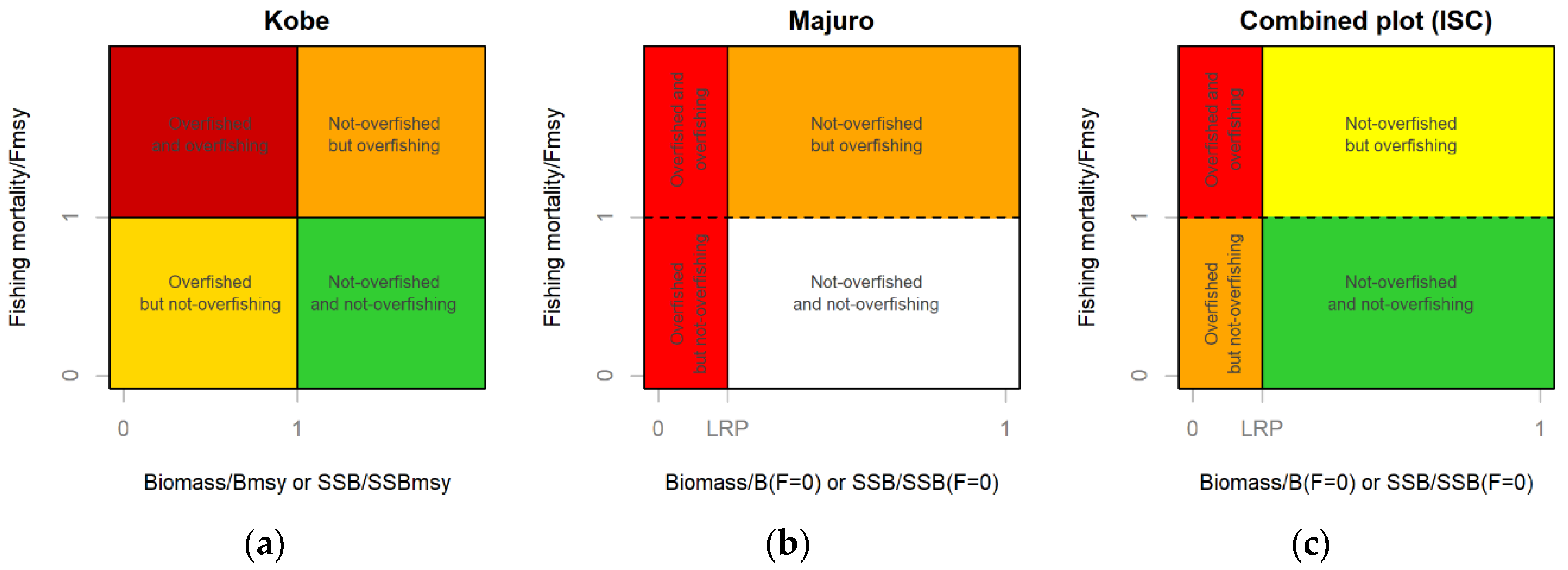
Three stock-status display conventions are relevant. A Kobe plot uses B/B_{MSY} or SSB/SSB_{MSY} on the biomass axis and F/F_{MSY} on the fishing-mortality axis. A Majuro plot keeps F/F_{MSY} on the fishing-mortality axis but replaces the biomass axis with depletion relative to unfished biomass, B/B_{F=0} or SSB/SSB_{F=0}. A combined plot overlays a limit-reference-point threshold on the unfished-biomass scale and uses color categories to distinguish low-biomass and high-fishing-mortality combinations (Merino et al., 2020).

The Majuro plot in this paper uses SSB/SSB_{F=0} from SSB_NoFishR and annual aggregate F divided by each run’s F_{MSY}. The vertical line at 0.2 is shown only as an orienting convention from WCPFC-style tuna displays. It is not proposed here as a jack mackerel limit reference point.

3 Results

3.1 Productivity Estimates

The F profile from h1_0.14ls provides the starting point for comparing MSY-based and SPR-based reference points. In Figure 1, F_{35\%} is marked against the same profile as F_{MSY}. The two values are close only under some productivity assumptions. Across all four runs, F_{35\%} is much more stable than F_{MSY} because it does not use the SRR.

Table 1: SPR reference point from h1_0.14ls. SBF35 is interpolated from the yield profile at SPR = 0.35.

model	stock	F35_est	F_at_SPR35_profile	Fmsy	SBF35	yield_at_SPR35	yield_at_Fmsy	SPR_at_Fmsy	recruitment_at_SPR35
h1_0.14ls	1	0.4621	0.4621	0.3148	3963.31	983.9154	1010.656	0.4224	7086.944

Figure 1: F profile from the h1_0.14ls yield-profile output. Vertical lines mark F35% and Fmsy on the profile.

Table 2: Fishery ratios used to apportion F-based reference points. Ratios are based on mean end-year F by fishery, matching the Fratio calculation used for SPR rates.

fishery	end_year	mean_f	max_selectivity_scaled_f	f_ratio	F35_est_contribution	F_at_SPR35_profile_contribution	Fmsy_contribution
N_Chile	2025	0.0383	0.0762	0.0490	0.0226	0.0226	0.0154
SC_Chile_PS	2025	0.7126	2.0406	0.9118	0.4213	0.4213	0.2871
FarNorth	2025	0.0240	0.0423	0.0307	0.0142	0.0142	0.0097
Offshore_Trawl	2025	0.0066	0.0137	0.0085	0.0039	0.0039	0.0027

The productivity sensitivity runs span F_{MSY} values from 0.315 to 0.878. The low-steepness cases define the lower end of the range, while the high-steepness cases shift the F-profile peak to substantially higher F values. Changing from the short to the long stock-recruit fitting period has a smaller effect within each steepness assumption than changing steepness itself.

Table 3: Fmsy values across productivity assumptions. Intervals use the reported standard errors from the .std files; profile_Fmsy is the F value at maximum yield in the yield profile.

model	scenario	steepness	sr_years	Fmsy	Fmsy_se	F35_est	F_at_SPR35_profile	Fcur_Fmsy	Bmsy	Bmsy_se	Bcur_Bmsy	profile_Fmsy	MSY	SPR_at_profile_Fmsy
h1_0.14ls	Low steepness, short SR	0.65	2001-2015	0.3148	0.0282	0.4621	0.4621	2.4822	5295.5	1341.00	1.1255	0.314	1010.660	0.4229
h1_0.14ll	Low steepness, long SR	0.65	1970-2022	0.3167	0.0279	0.4662	0.4662	2.5321	9130.4	1194.30	0.6424	0.316	1740.140	0.4233
h1_0.14hs	High steepness, short SR	0.85	2001-2015	0.8496	0.1360	0.4623	0.4623	0.9190	2572.2	468.40	2.3183	0.848	964.188	0.2536
h1_0.14hl	High steepness, long SR	0.85	1970-2022	0.8777	0.1389	0.4745	0.4745	0.9191	4653.5	472.11	1.2944	0.874	1747.210	0.2535

Figure 2: Fmsy and F35% estimates across productivity assumptions. Horizontal bars show approximate 95% intervals for Fmsy using the reported standard errors.

F35% is comparatively stable across these runs, ranging from 0.462 to 0.475. Under low steepness, F35% sits above F_{MSY}, so it would imply a more aggressive F than the production-based MSY estimate. Under high steepness, F_{MSY} is well above F35%, so F35% becomes the more conservative reference point.

Figure 3: Yield profiles across productivity assumptions. Colors identify productivity cases and line types identify the stock-recruit fitting period. Points mark the profile maximum and dashed vertical lines mark the reported Fmsy values.

3.2 Dynamic Bzero Estimates

The post-2000 view in Figure 4 shows that recent fished SSB trajectories are broadly similar across productivity cases, but the B_{MSY} reference levels diverge strongly. The low-steepness, long-SR run has the highest B_{MSY} (9130 kt), while the high-steepness, short-SR run has the lowest B_{MSY} (2572 kt). Consequently, status relative to B_{MSY} is strongly influenced by the productivity assumption.

Figure 4: Fished spawning biomass since 2000 across productivity assumptions. Dashed horizontal lines show Bmsy for each run.

The dynamic-Bzero comparison for h1_0.14ls is shown in Figure 5. This is a counterfactual SSB comparison: the no-fishing trajectory is not a fixed scalar but an annual dynamic series.

Figure 5: Estimated spawning biomass with fishing and the model counterfactual dynamic Bzero spawning biomass without fishing.

Figure 6: Spawning biomass depletion ratio estimated as fished spawning biomass divided by dynamic Bzero spawning biomass.

Table 4: Terminal-year dynamic-Bzero spawning-biomass comparison.

year	ssb_with_fishing	ssb_dynamic_bzero	dynamic_bzero_difference	ssb_over_dynamic_bzero	reported_depletion	ratio_minus_reported
2025	5960.19	18550.1	12589.91	0.3213	0.3213	0

3.3 Stock Status

Kobe, Majuro, and combined plots communicate different biomass-axis choices. Kobe plots divide biomass by B_{MSY}, so they can be sensitive to productivity assumptions when B_{MSY} changes. Majuro plots use depletion relative to unfished biomass, which can be easier to interpret when the working group wants to distinguish biomass depletion from the production-model estimate of B_{MSY}. Combined plots add a limit-reference-point threshold to the unfished-biomass scale while retaining the fishing-pressure axis (Figure 7).

Figure 7: Common stock-status display formats: Kobe, Majuro, and combined. Reproduced from Merino et al. (2020).

The Majuro plot in Figure 8 shows the 2000-2025 trajectory for each productivity case. Low-steepness runs end above F/F_{MSY} = 1, whereas high-steepness runs end just below 1. The biomass axis shows the same productivity contrast: terminal SSB/SSB_{F=0} is lower for the low-steepness runs (0.256-0.321) than for the high-steepness runs (0.402-0.431).

Figure 8: Majuro plot for model 0.14 productivity assumptions, showing the 2000-2025 trajectory. Larger points mark terminal-year status. The vertical line marks SSB/SSB_F=0 = 0.2 for orientation and the horizontal line marks F/Fmsy = 1.

Table 5: Terminal-year Majuro plot coordinates for the productivity sensitivity runs.

model	scenario	year	SSB_over_SSB_F0	F_over_Fmsy
h1_0.14ls	Low steepness, short SR	2025	0.3213	2.4822
h1_0.14ll	Low steepness, long SR	2025	0.2558	2.5322
h1_0.14hs	High steepness, short SR	2025	0.4312	0.9190
h1_0.14hl	High steepness, long SR	2025	0.4020	0.9191

4 Discussion

The working group has several options heading into the MSE workshop.

First, the MSE operating-model grid can retain explicit productivity uncertainty by conditioning operating models under low and high steepness and under short and long SRR fitting windows. That approach preserves the key biological uncertainty, but it requires clear rules about how reference points are calculated and held fixed during simulation.

Second, the working group can use SPR-based proxies such as F_{35\%} as candidate management-procedure reference points or as diagnostics alongside MSY-based quantities. SPR proxies do not remove uncertainty about selectivity, natural mortality, maturity, or growth, but they avoid direct dependence on the fitted SRR. This makes them useful when productivity assumptions are a central axis of the operating-model grid.

Third, the working group can use dynamic-Bzero and Majuro-style depletion displays to communicate stock status without requiring every biomass comparison to pass through B_{MSY}. This is especially useful here because the recent SSB trajectories are similar across productivity cases while B_{MSY} and F_{MSY} differ substantially.

The practical MSE choice is therefore not whether to keep or discard MSY-based reference points, but how to use them. A defensible near-term path is to carry MSY-based quantities as operating-model diagnostics, evaluate one or more SPR-based harvest-rate proxies as candidate management quantities, and use dynamic-Bzero depletion plots to communicate status across productivity cases. The final choice should be made after the working group agrees on which productivity cases enter the operating-model grid and whether reference points are fixed by draw, fixed by scenario, or recalculated during simulation.

References

Merino, G., Murua, H., Santiago, J., Arrizabalaga, H., & Restrepo, V. (2020). Characterization, communication, and management of uncertainty in tuna fisheries. Sustainability, 12(19), 8245. https://doi.org/10.3390/su12198245

SPRFMO Jack Mackerel Working Group. (2026a). Developments of the base SC13 model for benchmark and MSE considerations (SCW16/Paper-01). South Pacific Regional Fisheries Management Organisation (SPRFMO).

SPRFMO Jack Mackerel Working Group. (2026b). JMWG meeting report 01-2026. South Pacific Regional Fisheries Management Organisation (SPRFMO).

SPRFMO Scientific Committee. (2025). Annex 11: Jack mackerel technical annex. South Pacific Regional Fisheries Management Organisation (SPRFMO). https://sprfmo.int/assets/Meetings/02-SC/13th-SC-2025/SC13-Report-Annex-11_final.pdf