SCW17/Paper-06 Evaluation of indices for MP considerations

Published

June 16, 2026

1 Introduction

This working paper evaluates the abundance indices used in the h1_0.16 assessment configuration for SCW17 model development. The analysis is intended to identify whether retained indices provide broadly consistent information about relative abundance or whether some series move in opposing directions during overlapping years.

The index-correlation diagnostics focus on observed positive index values only. Chile_AcousCS is omitted, and the Chile_AcousN series is restricted to 2006 onward to avoid mixing the early acoustic-survey period with the modern survey period. Pairwise Pearson correlations are computed on log observed indices, while Spearman correlations are computed on the observed scale.

The final section uses the ROC/AUC diagnostic generated in the jmMSE repository (output/index_auc_h1_h2_0.16.rda, produced by output_auc_peru_cpue.R). Each index is evaluated as an indicator of annual changes in spawning stock biomass (SSB). The binary truth is whether SSB increased from the previous year, and the index score is the log annual index ratio. The area under the ROC curve (AUC) summarizes how well each index discriminates years of increasing SSB from years of non-increasing SSB.

2 Models

The report evaluates observed abundance indices in h1_0.16.ctl, omitting Chile_AcousCS and dropping Chile_AcousN years before 2006. Correlations are computed pairwise using only years where both indices have positive observations. Pearson correlations use log observed indices; Spearman correlations use the observed index values.

Table 1 identifies the model input and output files used for the index-correlation diagnostics. The retained index set and the filter applied to Chile_AcousN define the data used in all index-series and correlation figures below.

Table 2 gives the effective observation coverage after applying these filters. These counts are important when interpreting pairwise correlations because each contrast is calculated only over the years where both indices are available.

Table 1: Model file included in the index-correlation evaluation.

model	data_file	n_indices	indices	omitted_indices	notes	first_year	last_year
h1_0.16	0.15.dat	5	Chile_AcousN, Chile_CPUE, Peru_Artis, Peru_Ind, Offshore_CPUE	Chile_AcousCS	Chile_AcousN years before 2006 dropped	1970	2025

Table 2: Observed index coverage by model and index.

model	index	n	first_year	last_year	geometric_mean	min_observed	max_observed
h1_0.16	Chile_AcousN	19	2006	2025	465.816	18.000	3,058.843
h1_0.16	Chile_CPUE	28	1998	2025	91.845	59.322	147.633
h1_0.16	Offshore_CPUE	17	2008	2024	683.716	428.054	1,339.693
h1_0.16	Peru_Artis	24	2002	2025	0.263	0.079	0.672
h1_0.16	Peru_Ind	20	2002	2025	0.361	0.205	0.494

3 Index Series

Figure 1 shows the retained observed index series after rescaling each series to its own geometric mean. Chile_AcousN is shown in a separate lower panel because it is the only retained survey index and has a different scale from the CPUE-style indices; separating it makes the remaining index trajectories easier to compare. Figure 2 shows the same retained index series on an arithmetic y-axis after scaling each index to its own arithmetic mean; this view preserves the separate Chile_AcousN panel but avoids the compression introduced by the log scale.

Figure 1: Observed indices for h1_0.16, rescaled to each index’s geometric mean. Chile_AcousN is shown in a separate panel with its own y-axis scale.

Figure 2: Observed indices for h1_0.16, rescaled to each index’s arithmetic mean and shown on an arithmetic y-axis. Chile_AcousN is shown in a separate panel with its own y-axis scale.

4 Correlations

Figure 3 summarizes the pairwise Pearson correlations between log observed indices. The lower triangle gives the correlation coefficient for each pair: blue cells indicate positive correlations, red cells indicate negative correlations, and values closer to zero indicate weaker linear agreement over the overlapping years.

Table 3 gives the numerical values behind Figure 3 and also includes Spearman rank correlations on the observed scale. The overlap columns should be read alongside the coefficients because correlations based on short overlapping periods are less informative than those based on longer shared histories.

Figure 4 shows the underlying paired observations for each Pearson correlation. Each panel uses only years where both indices have positive observations, with point color indicating year and the grey line giving a simple linear fit on the log-index scale.

Figure 5 shows the same log-index data as a scatterplot matrix. Pearson correlations are printed in the upper triangle, while the lower triangle shows the paired observations with linear fits and uncertainty ribbons.

The pairwise overlap was largest for Chile_CPUE vs Peru_Artis, with 24 shared years. The lowest overlap was for Offshore_CPUE vs Peru_Ind, with 13 shared years. This difference in overlap should be considered when comparing the apparent strength of correlations across index pairs.

Figure 3: Pearson correlations between log observed indices after omitting Chile_AcousCS. Blue cells indicate positive correlations, red cells indicate negative correlations, and the lower triangle reports r for each pair.

Table 3: Pairwise index correlations. Pearson correlations use log observed indices; Spearman correlations use observed values. Pairs with fewer than the minimum overlapping years are reported as NA.

index_1	index_2	n_overlap	first_overlap	last_overlap	Correlation
index_1	index_2	n_overlap	first_overlap	last_overlap	Pearson	Spearman
Chile_AcousN	Peru_Artis	19	2006	2025	0.835	0.704
Peru_Artis	Peru_Ind	20	2002	2025	0.768	0.795
Chile_AcousN	Peru_Ind	15	2006	2025	0.767	0.650
Chile_CPUE	Offshore_CPUE	17	2008	2024	0.704	0.654
Offshore_CPUE	Peru_Ind	13	2008	2024	0.160	0.357
Chile_CPUE	Peru_Ind	20	2002	2025	−0.126	−0.343
Chile_AcousN	Chile_CPUE	19	2006	2025	0.095	0.042
Chile_AcousN	Offshore_CPUE	16	2008	2024	−0.064	0.109
Offshore_CPUE	Peru_Artis	17	2008	2024	0.045	0.042
Chile_CPUE	Peru_Artis	24	2002	2025	−0.036	−0.070

Figure 4: Pairwise index relationships for h1_0.16, excluding Chile_AcousCS. Axes are log observed indices and points are overlapping years used in the Pearson correlations.

Figure 5: Scatterplot matrix for log observed indices. Upper panels show Pearson correlations; lower panels show paired observations with linear fits and uncertainty ribbons.

5 Patterns in model fit residuals

The observation correlations above describe whether index observations move together. A complementary diagnostic is to compare model fit residuals, because shared residual patterns indicate years where indices contain similar information after the h1_0.16 model fit has already explained the common stock trend. This is more directly related to availability trade-offs among indices: two indices with strongly correlated residuals are likely to add less independent information than two indices whose residuals differ.

Table 4 gives the retained residual coverage by index for h1_0.16 and h2_0.16. Residuals are the standardized index-fit residuals reported in the JJM Obs_Survey_* output, after omitting Chile_AcousCS and dropping Chile_AcousN observations before 2006. Figure 6 shows the Pearson correlations among residuals for the one-stock hypothesis; Figure 7 shows the same diagnostic for the two-stock hypothesis.

Table 4: Model fit residual coverage by model and index. Residuals are standardized index-fit residuals from the JJM Obs_Survey output.

model	index	n	first_year	last_year	mean_residual	sd_residual
h1_0.16	Chile_AcousN	19	2006	2025	−2.248	8.756
h1_0.16	Chile_CPUE	28	1998	2025	−0.142	0.758
h1_0.16	Offshore_CPUE	17	2008	2024	−0.101	1.152
h1_0.16	Peru_Artis	24	2002	2025	−0.212	1.675
h1_0.16	Peru_Ind	20	2002	2025	−0.163	1.533
h2_0.16	Chile_AcousN	19	2006	2025	−2.300	9.088
h2_0.16	Chile_CPUE	28	1998	2025	−0.145	0.794
h2_0.16	Offshore_CPUE	17	2008	2024	−0.106	1.191
h2_0.16	Peru_Artis	24	2002	2025	−0.190	0.860
h2_0.16	Peru_Ind	20	2002	2025	−0.067	0.905

Figure 6: Pearson correlations between standardized model fit residuals for retained indices in h1_0.16. Blue cells indicate positive residual correlations and red cells indicate negative residual correlations.

For h2_0.16, the residual correlations span the two-stock model structure. The Peru_Artis and Peru_Ind residuals come from stock 2, while Chile_AcousN, Chile_CPUE, and Offshore_CPUE come from stock 1. Within stock 2, the residual correlation between Peru_Artis and Peru_Ind was -0.23 across 20 overlapping years (2002-2025). Pairs with strong positive residual correlations indicate indices that still tend to be high or low together after fitting their stock-specific trends; pairs closer to zero or negative values indicate more distinct residual information and may be more informative for availability trade-offs. Cross-stock residual correlations should therefore be read as comparisons between independently fitted stock components rather than as residuals from a single shared abundance trajectory.

Figure 7: Pearson correlations between standardized model fit residuals for retained indices in h2_0.16. Blue cells indicate positive residual correlations and red cells indicate negative residual correlations.

6 Index ROC/AUC

The ROC/AUC diagnostics below are loaded from the jmMSE output file output/index_auc_h1_h2_0.16.rda. They compare annual index changes against annual changes in model-estimated SSB. For each index, the score is $\log(I_y / I_{y-1})$ and the truth is whether $SSB_y > SSB_{y-1}$. For h1_0.16, each index is compared with the single-stock SSB trajectory. For h2_0.16, each index is compared with the SSB trajectory for the stock-specific output block in which the index appears. The Chile_AcousN ROC diagnostic uses only observations after 2005, following the implementation in jmMSE/output_auc_peru_cpue.R.

Figure 8 shows the h1 single-stock ROC diagnostics. Curves above the one-to-one dashed line indicate that positive index changes tend to coincide with years when model-estimated SSB increased; AUC values closer to one indicate stronger discrimination.

Figure 9 applies the same diagnostic to the h2 stock-specific outputs. The southern-stock indices and northern-stock indices are evaluated against their corresponding stock-specific SSB changes, so these panels should not be interpreted as a single pooled-stock diagnostic.

Table 5 summarizes the AUC and number of annual index changes used in each ROC curve from Figure 8 and Figure 9.

Figure 8: Receiver Operating Characteristic (ROC) curves for abundance indices as indicators of changes in spawning stock biomass (SSB) in h1_0.16. Chile_AcousN uses only observations after 2005.

Figure 9: Receiver Operating Characteristic (ROC) curves for abundance indices as indicators of changes in stock-specific spawning stock biomass (SSB) in h2_0.16. Chile_AcousN uses only observations after 2005.

Table 5: Index ROC/AUC summaries for h1_0.16 and h2_0.16. The truth is annual SSB direction and the score is the annual log index ratio.

model	stock	index	n	auc
h1_0.16	single stock	Offshore_CPUE	16	0.933
h1_0.16	single stock	Chile_CPUE	27	0.672
h1_0.16	single stock	Chile_AcousCS	12	0.657
h1_0.16	single stock	Chile_AcousN	18	0.525
h1_0.16	single stock	Peru_Artis	23	0.485
h1_0.16	single stock	Peru_Ind	19	0.443
h2_0.16	northern stock	Peru_Ind	19	0.933
h2_0.16	northern stock	Peru_Artis	23	0.882
h2_0.16	southern stock	Offshore_CPUE	16	0.821
h2_0.16	southern stock	Chile_CPUE	27	0.724
h2_0.16	southern stock	Chile_AcousCS	12	0.583
h2_0.16	southern stock	Chile_AcousN	18	0.508

7 Summary

Table 6 extracts the largest positive and most negative Pearson correlations from the correlation table. This is a compact way to identify the index pairs with the strongest agreement and strongest disagreement after accounting for the available overlapping years.

This evaluation shows that, for the two-stock hypotheses, the nominal CPUE indices for Peru generally track stock trends. Those same indices perform relatively poorer under the single-stock hypothesis. For the single-stock case, the offshore CPUE and Chilean CPUE indices appear to perform better. These conclusions are broadly consistent between the pairwise index comparisons and the ROC/AUC evaluations.

Table 7 reports the covariance matrix used to simulate the multivariate index draws in long form. Figure 10 uses that estimated correlation structure among the retained index series to simulate 100 multivariate draws. The simulation uses the Pearson correlations among log observed indices for Chile_AcousN, Chile_CPUE, Offshore_CPUE, Peru_Artis, and Peru_Ind; the diagonal uncertainty is set to 20% CV for all indices except the two Peruvian CPUE series, which use 30% CV.

Table 8 and Table 9 report the fitted-residual covariance structures used for residual-based simulations. Figure 11 and Figure 12 use the residual covariance among retained indices for h1_0.16 and h2_0.16, respectively. In these residual-based simulations, the diagonal is not externally specified; it is the empirical variance of the model fit residuals for each index.

Table 6: Strongest positive and negative contrasts. Based on Pearson correlations of log-observed indices.

index_1	index_2	n_overlap	first_overlap	last_overlap	correlation
Chile_AcousN	Peru_Artis	19	2006	2025	0.835
Peru_Artis	Peru_Ind	20	2002	2025	0.768
Chile_AcousN	Peru_Ind	15	2006	2025	0.767
Chile_CPUE	Peru_Artis	24	2002	2025	−0.036
Chile_AcousN	Offshore_CPUE	16	2008	2024	−0.064
Chile_CPUE	Peru_Ind	20	2002	2025	−0.126

Table 7: Long-form covariance matrix used to generate the simulated multivariate index draws. Covariances are on the log-index multiplier scale after converting specified CVs to log-scale standard deviations.

index_1	index_2	cv_1	cv_2	correlation	covariance
Chile_AcousN	Chile_AcousN	20%	20%	1.0000	0.0392
Chile_AcousN	Chile_CPUE	20%	20%	0.0951	0.0037
Chile_AcousN	Offshore_CPUE	20%	20%	−0.0642	−0.0025
Chile_AcousN	Peru_Artis	20%	30%	0.8352	0.0486
Chile_AcousN	Peru_Ind	20%	30%	0.7668	0.0446
Chile_CPUE	Chile_AcousN	20%	20%	0.0951	0.0037
Chile_CPUE	Chile_CPUE	20%	20%	1.0000	0.0392
Chile_CPUE	Offshore_CPUE	20%	20%	0.7041	0.0276
Chile_CPUE	Peru_Artis	20%	30%	−0.0361	−0.0021
Chile_CPUE	Peru_Ind	20%	30%	−0.1257	−0.0073
Offshore_CPUE	Chile_AcousN	20%	20%	−0.0642	−0.0025
Offshore_CPUE	Chile_CPUE	20%	20%	0.7041	0.0276
Offshore_CPUE	Offshore_CPUE	20%	20%	1.0000	0.0392
Offshore_CPUE	Peru_Artis	20%	30%	0.0452	0.0026
Offshore_CPUE	Peru_Ind	20%	30%	0.1605	0.0093
Peru_Artis	Chile_AcousN	30%	20%	0.8352	0.0486
Peru_Artis	Chile_CPUE	30%	20%	−0.0361	−0.0021
Peru_Artis	Offshore_CPUE	30%	20%	0.0452	0.0026
Peru_Artis	Peru_Artis	30%	30%	1.0000	0.0862
Peru_Artis	Peru_Ind	30%	30%	0.7682	0.0662
Peru_Ind	Chile_AcousN	30%	20%	0.7668	0.0446
Peru_Ind	Chile_CPUE	30%	20%	−0.1257	−0.0073
Peru_Ind	Offshore_CPUE	30%	20%	0.1605	0.0093
Peru_Ind	Peru_Artis	30%	30%	0.7682	0.0662
Peru_Ind	Peru_Ind	30%	30%	1.0000	0.0862

Figure 10: Simulated multivariate index draws using the estimated correlation structure among retained indices. Diagonal uncertainty assumes 20% CV except Peru_Artis and Peru_Ind, which use 30% CV.

Table 8: Long-form covariance matrix used to generate simulated residual draws for h1_0.16. Covariances are computed from standardized index-fit residuals.

model	index_1	index_2	n_overlap	correlation	covariance
h1_0.16	Chile_AcousN	Chile_AcousN	19	1.0000	76.6691
h1_0.16	Chile_AcousN	Chile_CPUE	19	−0.2101	−1.5750
h1_0.16	Chile_AcousN	Offshore_CPUE	16	−0.2622	−2.7772
h1_0.16	Chile_AcousN	Peru_Artis	19	0.2798	1.8054
h1_0.16	Chile_AcousN	Peru_Ind	15	−0.2065	−2.5659
h1_0.16	Chile_CPUE	Chile_AcousN	19	−0.2101	−1.5750
h1_0.16	Chile_CPUE	Chile_CPUE	28	1.0000	0.5748
h1_0.16	Chile_CPUE	Offshore_CPUE	17	0.0425	0.0440
h1_0.16	Chile_CPUE	Peru_Artis	24	−0.0580	−0.0793
h1_0.16	Chile_CPUE	Peru_Ind	20	0.1157	0.1101
h1_0.16	Offshore_CPUE	Chile_AcousN	16	−0.2622	−2.7772
h1_0.16	Offshore_CPUE	Chile_CPUE	17	0.0425	0.0440
h1_0.16	Offshore_CPUE	Offshore_CPUE	17	1.0000	1.3260
h1_0.16	Offshore_CPUE	Peru_Artis	17	−0.2149	−0.1873
h1_0.16	Offshore_CPUE	Peru_Ind	13	0.2652	0.4330
h1_0.16	Peru_Artis	Chile_AcousN	19	0.2798	1.8054
h1_0.16	Peru_Artis	Chile_CPUE	24	−0.0580	−0.0793
h1_0.16	Peru_Artis	Offshore_CPUE	17	−0.2149	−0.1873
h1_0.16	Peru_Artis	Peru_Artis	24	1.0000	2.8068
h1_0.16	Peru_Artis	Peru_Ind	20	0.5525	1.5500
h1_0.16	Peru_Ind	Chile_AcousN	15	−0.2065	−2.5659
h1_0.16	Peru_Ind	Chile_CPUE	20	0.1157	0.1101
h1_0.16	Peru_Ind	Offshore_CPUE	13	0.2652	0.4330
h1_0.16	Peru_Ind	Peru_Artis	20	0.5525	1.5500
h1_0.16	Peru_Ind	Peru_Ind	20	1.0000	2.3499

Figure 11: Simulated multivariate residual draws for h1_0.16 using the estimated covariance structure among retained index fit residuals. Diagonal uncertainty is the empirical residual variance for each index.

Table 9: Long-form covariance matrix used to generate simulated residual draws for h2_0.16. Covariances are computed from standardized index-fit residuals.

model	index_1	index_2	n_overlap	correlation	covariance
h2_0.16	Chile_AcousN	Chile_AcousN	19	1.0000	82.5922
h2_0.16	Chile_AcousN	Chile_CPUE	19	−0.2004	−1.6474
h2_0.16	Chile_AcousN	Offshore_CPUE	16	−0.1972	−2.2536
h2_0.16	Chile_AcousN	Peru_Artis	19	0.2900	2.1971
h2_0.16	Chile_AcousN	Peru_Ind	15	−0.3687	−3.1899
h2_0.16	Chile_CPUE	Chile_AcousN	19	−0.2004	−1.6474
h2_0.16	Chile_CPUE	Chile_CPUE	28	1.0000	0.6309
h2_0.16	Chile_CPUE	Offshore_CPUE	17	0.0629	0.0705
h2_0.16	Chile_CPUE	Peru_Artis	24	−0.2447	−0.1804
h2_0.16	Chile_CPUE	Peru_Ind	20	0.0133	0.0077
h2_0.16	Offshore_CPUE	Chile_AcousN	16	−0.1972	−2.2536
h2_0.16	Offshore_CPUE	Chile_CPUE	17	0.0629	0.0705
h2_0.16	Offshore_CPUE	Offshore_CPUE	17	1.0000	1.4187
h2_0.16	Offshore_CPUE	Peru_Artis	17	−0.4201	−0.4006
h2_0.16	Offshore_CPUE	Peru_Ind	13	0.1237	0.1500
h2_0.16	Peru_Artis	Chile_AcousN	19	0.2900	2.1971
h2_0.16	Peru_Artis	Chile_CPUE	24	−0.2447	−0.1804
h2_0.16	Peru_Artis	Offshore_CPUE	17	−0.4201	−0.4006
h2_0.16	Peru_Artis	Peru_Artis	24	1.0000	0.7397
h2_0.16	Peru_Artis	Peru_Ind	20	−0.2272	−0.1929
h2_0.16	Peru_Ind	Chile_AcousN	15	−0.3687	−3.1899
h2_0.16	Peru_Ind	Chile_CPUE	20	0.0133	0.0077
h2_0.16	Peru_Ind	Offshore_CPUE	13	0.1237	0.1500
h2_0.16	Peru_Ind	Peru_Artis	20	−0.2272	−0.1929
h2_0.16	Peru_Ind	Peru_Ind	20	1.0000	0.8189

Figure 12: Simulated multivariate residual draws for h2_0.16 using the estimated covariance structure among retained index fit residuals. Diagonal uncertainty is the empirical residual variance for each index.

--- title: "SCW17/Paper-06 Evaluation of indices for MP considerations" date: today format: html: output-file: "SCW17-Paper-06-Evaluation-of-indices-for-MP-considerations.html" toc: true toc-depth: 3 number-sections: true code-fold: true code-tools: true df-print: paged theme: cosmo fig-width: 9 fig-height: 5 lightbox: true execute: warning: false message: false params: index_models: - "h1_0.16" auc_models: - "h1_0.16" - "h2_0.16" omit_indices: - "Chile_AcousCS" chile_acousn_start_year: 2006 min_overlap: 3 assessment_path: "../../jjm/assessment" jmMSE_path: "../../jmMSE" --- ```{r} #| label: setup #| include: false library(jjmR) library(dplyr) library(GGally) library(ggplot2) library(ggcorrplot) library(ggthemes) library(gt) library(purrr) library(tidyr) index_model_names <- unlist(params$index_models) auc_model_names <- unlist(params$auc_models) all_model_names <- union(index_model_names, auc_model_names) omit_indices <- unlist(params$omit_indices) chile_acousn_start_year <- params$chile_acousn_start_year assessment_path <- params$assessment_path jmMSE_path <- params$jmMSE_path read_model <- function(model_name) { readJJM( model_name, path = file.path(assessment_path, "config"), input = file.path(assessment_path, "input"), output = file.path(assessment_path, "results"), version = "2015MS" )[[1]] } available_models <- all_model_names[ file.exists(file.path(assessment_path, "config", paste0(all_model_names, ".ctl"))) & file.exists(file.path(assessment_path, "results", paste0(all_model_names, ".rep"))) ] mods <- setNames(map(available_models, read_model), available_models) index_models <- intersect(index_model_names, available_models) auc_models <- intersect(auc_model_names, available_models) residual_models <- auc_models theme_report <- function() { theme_minimal(base_size = 12) + theme( legend.position = "top", panel.grid.minor = element_blank(), plot.title.position = "plot" ) } ggpairs_lower_lm <- function(data, mapping, ...) { ggplot(data = data, mapping = mapping) + geom_point(alpha = 0.7, size = 0.8, na.rm = TRUE) + geom_smooth(method = "lm", se = TRUE, color = "grey30", fill = "grey70", linewidth = 0.4, na.rm = TRUE) + ggthemes::theme_few(base_size = 9) } model_index_df <- function(model_name) { dat <- mods[[model_name]]$data index_mat <- dat$Index colnames(index_mat) <- dat$Inames as_tibble(index_mat, rownames = "year") |> mutate(year = as.integer(year), model = model_name, .before = 1) |> pivot_longer( cols = -c(model, year), names_to = "index", values_to = "observed" ) |> filter( !index %in% omit_indices, index != "Chile_AcousN" | year >= chile_acousn_start_year, !is.na(observed), observed > 0 ) |> group_by(model, index) |> mutate( log_observed = log(observed), relative_index = observed / exp(mean(log_observed, na.rm = TRUE)), relative_index_arithmetic = observed / mean(observed, na.rm = TRUE), z_log_index = as.numeric(scale(log_observed)) ) |> ungroup() } index_data <- map_dfr(index_models, model_index_df) model_index_residual_df <- function(model_name) { dat <- mods[[model_name]]$data outputs <- mods[[model_name]]$output map_dfr(outputs, function(out) { obs_survey_names <- grep("^Obs_Survey_", names(out), value = TRUE) index_names <- as.vector(out$Index_names) map_dfr(seq_along(obs_survey_names), function(i) { survey_number <- as.integer(sub("^Obs_Survey_", "", obs_survey_names[[i]])) index_name <- if (i <= length(index_names)) { index_names[[i]] } else { dat$Inames[[survey_number]] } x <- as_tibble(out[[obs_survey_names[[i]]]], .name_repair = "unique") if (ncol(x) < 5) { return(NULL) } names(x)[seq_len(5)] <- c("year", "observed", "fitted", "sd", "fit_residual") x |> transmute( model = model_name, index = index_name, year = as.integer(year), observed = as.numeric(observed), fitted = as.numeric(fitted), sd = as.numeric(sd), fit_residual = as.numeric(fit_residual) ) |> filter( !index %in% omit_indices, index != "Chile_AcousN" | year >= chile_acousn_start_year, is.finite(fit_residual), observed > 0, fitted > 0 ) }) }) } index_residual_data <- map_dfr(residual_models, model_index_residual_df) model_summary <- map_dfr(index_models, function(model_name) { dat <- mods[[model_name]]$data tibble( model = model_name, data_file = mods[[model_name]]$control$dataFile, n_indices = sum(!dat$Inames %in% omit_indices), indices = paste(setdiff(dat$Inames, omit_indices), collapse = ", "), omitted_indices = paste(intersect(dat$Inames, omit_indices), collapse = ", "), notes = paste0("Chile_AcousN years before ", chile_acousn_start_year, " dropped"), first_year = min(as.integer(rownames(dat$Index)), na.rm = TRUE), last_year = max(as.integer(rownames(dat$Index)), na.rm = TRUE) ) }) jmMSE_roc_file <- file.path(jmMSE_path, "output", "index_auc_h1_h2_0.16.rda") if (!file.exists(jmMSE_roc_file)) { stop( "jmMSE ROC/AUC object not found: ", jmMSE_roc_file, "\nRun jmMSE/output_auc_peru_cpue.R first.", call. = FALSE ) } load(jmMSE_roc_file) h1_index_roc <- as_tibble(h1_roc) |> rename(index = survey) h2_index_roc <- as_tibble(h2_roc) |> rename(index = survey) index_roc_summary <- bind_rows(h1_index_roc, h2_index_roc) |> group_by(model, stock, index) |> summarise( n = first(n), auc = first(auc), .groups = "drop" ) index_summary <- index_data |> group_by(model, index) |> summarise( n = n(), first_year = min(year), last_year = max(year), geometric_mean = exp(mean(log_observed)), min_observed = min(observed), max_observed = max(observed), .groups = "drop" ) pairwise_correlations <- function(dat, value_col, method = "pearson") { indices <- sort(unique(dat$index)) pairs <- t(combn(indices, 2)) map_dfr(seq_len(nrow(pairs)), function(i) { x_name <- pairs[i, 1] y_name <- pairs[i, 2] pair_dat <- dat |> filter(index %in% c(x_name, y_name)) |> select(year, index, value = all_of(value_col)) |> pivot_wider(names_from = index, values_from = value) |> filter(!is.na(.data[[x_name]]), !is.na(.data[[y_name]])) tibble( index_1 = x_name, index_2 = y_name, n_overlap = nrow(pair_dat), first_overlap = if_else(nrow(pair_dat) > 0, min(pair_dat$year), NA_integer_), last_overlap = if_else(nrow(pair_dat) > 0, max(pair_dat$year), NA_integer_), correlation = if_else( nrow(pair_dat) >= params$min_overlap, cor(pair_dat[[x_name]], pair_dat[[y_name]], method = method), NA_real_ ) ) }) } pairwise_points <- function(dat) { indices <- sort(unique(dat$index)) pairs <- t(combn(indices, 2)) map_dfr(seq_len(nrow(pairs)), function(i) { x_name <- pairs[i, 1] y_name <- pairs[i, 2] dat |> filter(index %in% c(x_name, y_name)) |> select(year, index, log_observed) |> pivot_wider(names_from = index, values_from = log_observed) |> filter(!is.na(.data[[x_name]]), !is.na(.data[[y_name]])) |> transmute( index_1 = x_name, index_2 = y_name, pair = paste(x_name, y_name, sep = " vs "), year = year, x = .data[[x_name]], y = .data[[y_name]] ) }) } correlation_results <- index_data |> group_by(model) |> group_modify(\(.x, .y) { bind_rows( pairwise_correlations(.x, "log_observed", "pearson") |> mutate(scale = "log observed", method = "Pearson"), pairwise_correlations(.x, "observed", "spearman") |> mutate(scale = "observed", method = "Spearman") ) }) |> ungroup() |> select(model, method, scale, index_1, index_2, n_overlap, first_overlap, last_overlap, correlation) correlation_table <- correlation_results |> select(method, index_1, index_2, n_overlap, first_overlap, last_overlap, correlation) |> pivot_wider(names_from = method, values_from = correlation) |> arrange(desc(abs(Pearson)), index_1, index_2) heatmap_data <- correlation_results |> filter(method == "Pearson", scale == "log observed") |> mutate( pair = paste(index_1, index_2, sep = " vs "), label = if_else(is.na(correlation), "NA", sprintf("%.2f", correlation)) ) overlap_summary <- heatmap_data |> filter(!is.na(n_overlap)) |> summarise( max_overlap = max(n_overlap), min_overlap = min(n_overlap), max_pairs = paste(pair[n_overlap == max_overlap], collapse = "; "), min_pairs = paste(pair[n_overlap == min_overlap], collapse = "; ") ) correlation_matrix <- index_data |> select(year, index, log_observed) |> pivot_wider(names_from = index, values_from = log_observed) |> select(-year) |> as.data.frame() |> cor(use = "pairwise.complete.obs", method = "pearson") pair_matrix_data <- index_data |> select(year, index, log_observed) |> pivot_wider(names_from = index, values_from = log_observed) |> select(-year) pair_plot_data <- index_data |> group_by(model) |> group_modify(\(.x, .y) pairwise_points(.x)) |> ungroup() |> left_join( heatmap_data |> select(model, index_1, index_2, correlation, n_overlap), by = c("model", "index_1", "index_2") ) covariance_indices <- c("Chile_AcousN", "Chile_CPUE", "Offshore_CPUE", "Peru_Artis", "Peru_Ind") covariance_cvs <- c( Chile_AcousN = 0.20, Chile_CPUE = 0.20, Offshore_CPUE = 0.20, Peru_Artis = 0.30, Peru_Ind = 0.30 ) covariance_correlation <- correlation_matrix[covariance_indices, covariance_indices] covariance_correlation[is.na(covariance_correlation)] <- 0 diag(covariance_correlation) <- 1 make_positive_definite <- function(x, epsilon = 1e-8) { eigen_decomp <- eigen(x, symmetric = TRUE) eigen_decomp$vectors %*% diag(pmax(eigen_decomp$values, epsilon), nrow = length(eigen_decomp$values)) %*% t(eigen_decomp$vectors) } covariance_sdlog <- sqrt(log1p(covariance_cvs[covariance_indices]^2)) index_covariance <- diag(covariance_sdlog) %*% make_positive_definite(as.matrix(covariance_correlation)) %*% diag(covariance_sdlog) dimnames(index_covariance) <- list(covariance_indices, covariance_indices) covariance_matrix_long <- expand_grid( index_1 = covariance_indices, index_2 = covariance_indices ) |> mutate( cv_1 = unname(covariance_cvs[index_1]), cv_2 = unname(covariance_cvs[index_2]), correlation = as.numeric(covariance_correlation[cbind(index_1, index_2)]), covariance = as.numeric(index_covariance[cbind(index_1, index_2)]) ) set.seed(20260615) index_covariance_draws <- matrix( rnorm(100 * length(covariance_indices)), nrow = 100, ncol = length(covariance_indices) ) %*% chol(index_covariance) index_covariance_draws <- sweep( index_covariance_draws, 2, -0.5 * covariance_sdlog^2, "+" ) |> exp() |> as_tibble(.name_repair = "minimal") names(index_covariance_draws) <- covariance_indices residual_summary <- index_residual_data |> group_by(model, index) |> summarise( n = n(), first_year = min(year), last_year = max(year), mean_residual = mean(fit_residual), sd_residual = sd(fit_residual), .groups = "drop" ) residual_correlation_matrix <- function(model_name) { index_residual_data |> filter(model == model_name, index %in% covariance_indices) |> select(year, index, fit_residual) |> pivot_wider(names_from = index, values_from = fit_residual) |> select(any_of(covariance_indices)) |> as.data.frame() |> cor(use = "pairwise.complete.obs", method = "pearson") } h1_residual_correlation_matrix <- residual_correlation_matrix("h1_0.16") h2_residual_correlation_matrix <- residual_correlation_matrix("h2_0.16") residual_wide <- function(model_name) { index_residual_data |> filter(model == model_name, index %in% covariance_indices) |> select(year, index, fit_residual) |> pivot_wider(names_from = index, values_from = fit_residual) |> select(any_of(covariance_indices)) } residual_covariance_matrix <- function(model_name) { residual_wide(model_name) |> as.data.frame() |> cov(use = "pairwise.complete.obs") } residual_overlap_matrix <- function(model_name) { wide <- residual_wide(model_name) indices <- names(wide) expand_grid(index_1 = indices, index_2 = indices) |> mutate( n_overlap = map2_int( index_1, index_2, \(x, y) sum(!is.na(wide[[x]]) & !is.na(wide[[y]])) ) ) } residual_covariance_long <- function(model_name, covariance_matrix, correlation_matrix) { residual_overlap_matrix(model_name) |> mutate( model = model_name, correlation = as.numeric(correlation_matrix[cbind(index_1, index_2)]), covariance = as.numeric(covariance_matrix[cbind(index_1, index_2)]) ) |> select(model, index_1, index_2, n_overlap, correlation, covariance) } simulate_residual_covariance_draws <- function(covariance_matrix, seed) { set.seed(seed) draw_matrix <- matrix( rnorm(100 * ncol(covariance_matrix)), nrow = 100, ncol = ncol(covariance_matrix) ) %*% chol(make_positive_definite(as.matrix(covariance_matrix))) as_tibble(draw_matrix, .name_repair = "minimal") |> set_names(colnames(covariance_matrix)) } h1_residual_covariance_matrix <- residual_covariance_matrix("h1_0.16") h2_residual_covariance_matrix <- residual_covariance_matrix("h2_0.16") h1_residual_covariance_long <- residual_covariance_long( "h1_0.16", h1_residual_covariance_matrix, h1_residual_correlation_matrix ) h2_residual_covariance_long <- residual_covariance_long( "h2_0.16", h2_residual_covariance_matrix, h2_residual_correlation_matrix ) h1_residual_covariance_draws <- simulate_residual_covariance_draws( h1_residual_covariance_matrix, 20260616 ) h2_residual_covariance_draws <- simulate_residual_covariance_draws( h2_residual_covariance_matrix, 20260617 ) h2_stock2_residual_pair <- index_residual_data |> filter(model == "h2_0.16", index %in% c("Peru_Artis", "Peru_Ind")) |> select(year, index, fit_residual) |> pivot_wider(names_from = index, values_from = fit_residual) |> filter(!is.na(Peru_Artis), !is.na(Peru_Ind)) h2_stock2_residual_correlation <- cor( h2_stock2_residual_pair$Peru_Artis, h2_stock2_residual_pair$Peru_Ind ) ``` {{< include _includes/sprfmo-banner.html >}} ```{=html} <div class="paper-title">SCW17/Paper-06 Evaluation of indices for MP considerations</div> ``` ## Introduction This working paper evaluates the abundance indices used in the `h1_0.16` assessment configuration for SCW17 model development. The analysis is intended to identify whether retained indices provide broadly consistent information about relative abundance or whether some series move in opposing directions during overlapping years. The index-correlation diagnostics focus on observed positive index values only. `Chile_AcousCS` is omitted, and the `Chile_AcousN` series is restricted to 2006 onward to avoid mixing the early acoustic-survey period with the modern survey period. Pairwise Pearson correlations are computed on log observed indices, while Spearman correlations are computed on the observed scale. The final section uses the ROC/AUC diagnostic generated in the `jmMSE` repository (`output/index_auc_h1_h2_0.16.rda`, produced by `output_auc_peru_cpue.R`). Each index is evaluated as an indicator of annual changes in spawning stock biomass (SSB). The binary truth is whether SSB increased from the previous year, and the index score is the log annual index ratio. The area under the ROC curve (AUC) summarizes how well each index discriminates years of increasing SSB from years of non-increasing SSB. ## Models The report evaluates observed abundance indices in `h1_0.16.ctl`, omitting `Chile_AcousCS` and dropping `Chile_AcousN` years before 2006. Correlations are computed pairwise using only years where both indices have positive observations. Pearson correlations use log observed indices; Spearman correlations use the observed index values. @tbl-model-summary identifies the model input and output files used for the index-correlation diagnostics. The retained index set and the filter applied to `Chile_AcousN` define the data used in all index-series and correlation figures below. @tbl-index-summary gives the effective observation coverage after applying these filters. These counts are important when interpreting pairwise correlations because each contrast is calculated only over the years where both indices are available. 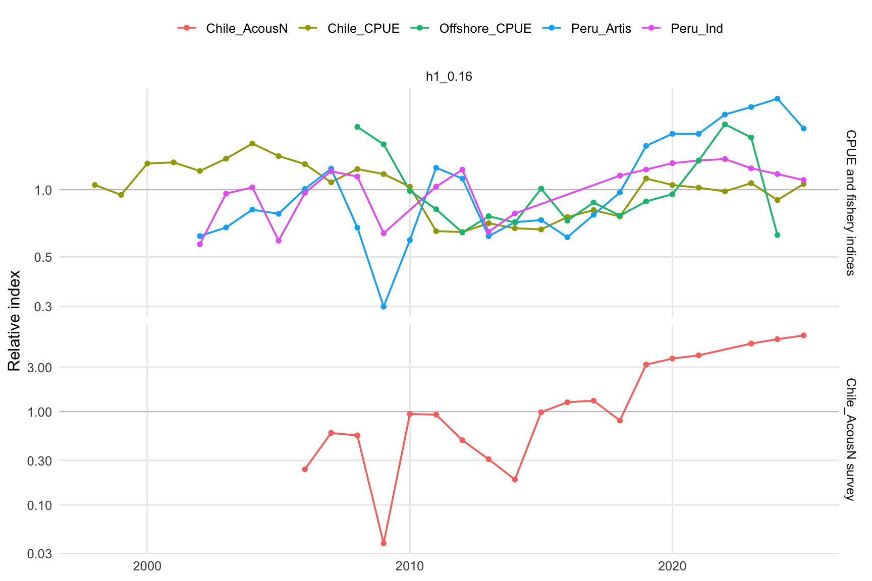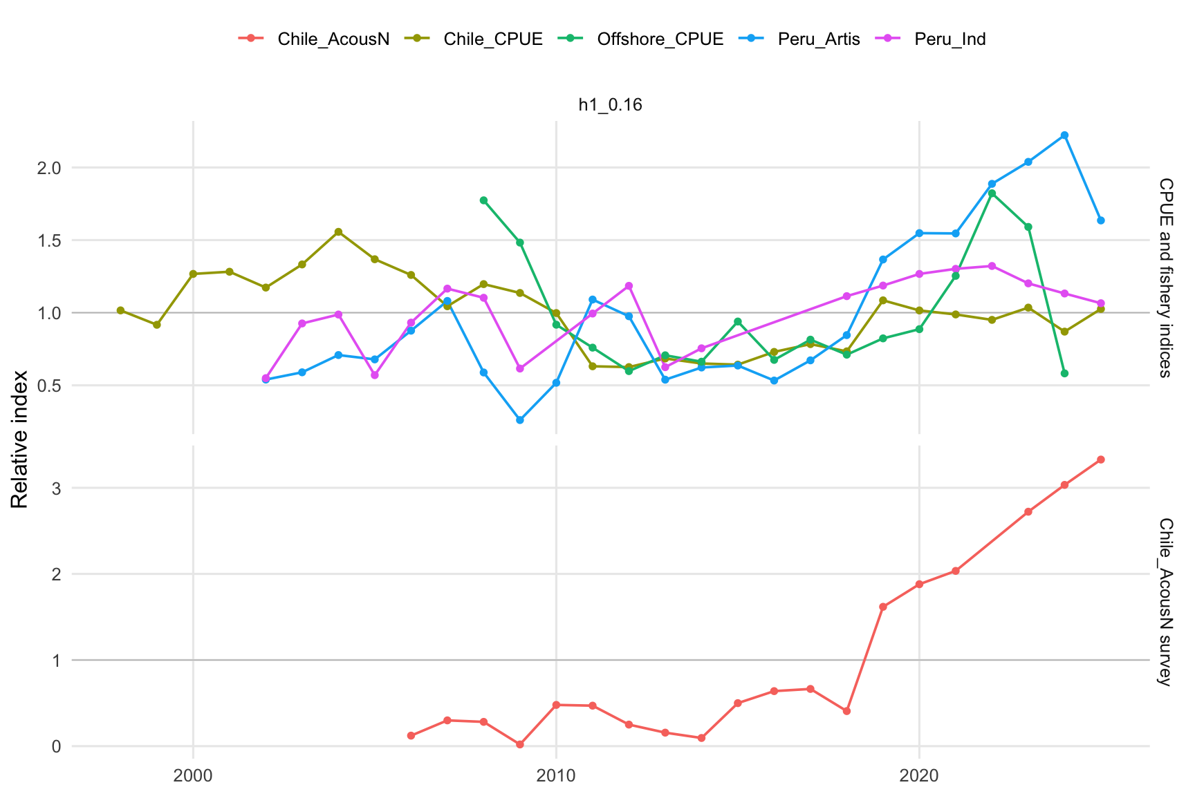```{r} #| label: tbl-model-summary #| tbl-cap: "Model file included in the index-correlation evaluation." #| echo: false model_summary |> gt() ``` ```{r} #| label: tbl-index-summary #| tbl-cap: "Observed index coverage by model and index." #| echo: false index_summary |> gt() |> fmt_number(columns = c(geometric_mean, min_observed, max_observed), decimals = 3) ``` ## Index Series @fig-relative-index-series shows the retained observed index series after rescaling each series to its own geometric mean. `Chile_AcousN` is shown in a separate lower panel because it is the only retained survey index and has a different scale from the CPUE-style indices; separating it makes the remaining index trajectories easier to compare. @fig-relative-index-series-arithmetic shows the same retained index series on an arithmetic y-axis after scaling each index to its own arithmetic mean; this view preserves the separate `Chile_AcousN` panel but avoids the compression introduced by the log scale. ```{r} #| label: fig-relative-index-series #| fig-cap: "Observed indices for h1_0.16, rescaled to each index's geometric mean. Chile_AcousN is shown in a separate panel with its own y-axis scale." #| echo: false #| fig-height: 6 index_data |> mutate( index_panel = if_else( index == "Chile_AcousN", "Chile_AcousN survey", "CPUE and fishery indices" ), index_panel = factor(index_panel, levels = c("CPUE and fishery indices", "Chile_AcousN survey")) ) |> ggplot(aes(year, relative_index, color = index)) + geom_hline(yintercept = 1, color = "grey75", linewidth = 0.3) + geom_line(linewidth = 0.65) + geom_point(size = 1.3) + facet_grid(index_panel ~ model, scales = "free_y") + scale_y_log10() + labs(x = NULL, y = "Relative index", color = NULL) + theme_report() ``` ```{r} #| label: fig-relative-index-series-arithmetic #| fig-cap: "Observed indices for h1_0.16, rescaled to each index's arithmetic mean and shown on an arithmetic y-axis. Chile_AcousN is shown in a separate panel with its own y-axis scale." #| echo: false #| fig-height: 6 index_data |> mutate( index_panel = if_else( index == "Chile_AcousN", "Chile_AcousN survey", "CPUE and fishery indices" ), index_panel = factor(index_panel, levels = c("CPUE and fishery indices", "Chile_AcousN survey")) ) |> ggplot(aes(year, relative_index_arithmetic, color = index)) + geom_hline(yintercept = 1, color = "grey75", linewidth = 0.3) + geom_line(linewidth = 0.65) + geom_point(size = 1.3) + facet_grid(index_panel ~ model, scales = "free_y") + labs(x = NULL, y = "Relative index", color = NULL) + theme_report() ``` ## Correlations @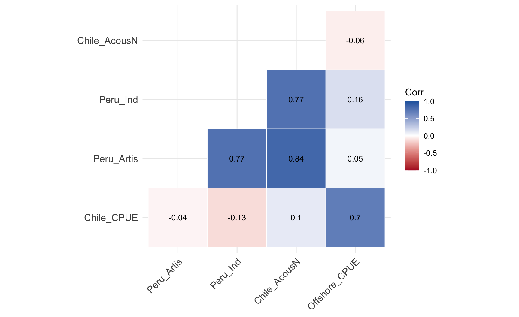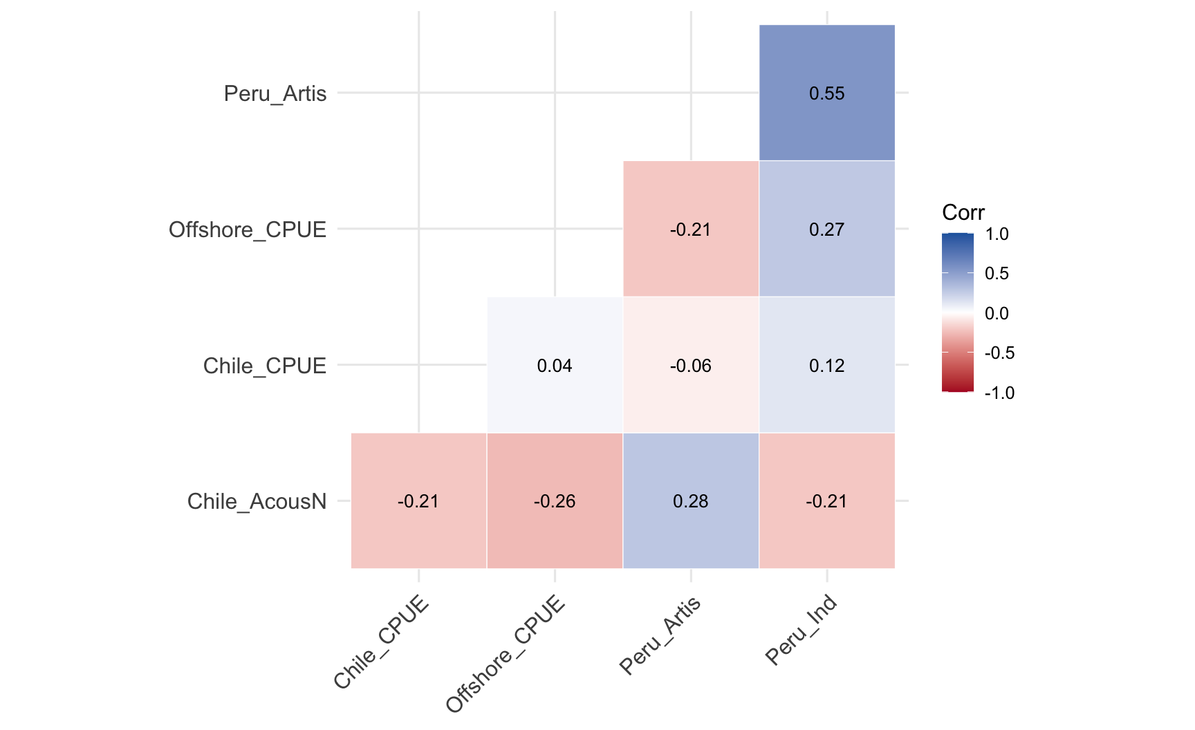fig-correlation-heatmap summarizes the pairwise Pearson correlations between log observed indices. The lower triangle gives the correlation coefficient for each pair: blue cells indicate positive correlations, red cells indicate negative correlations, and values closer to zero indicate weaker linear agreement over the overlapping years. @tbl-correlations gives the numerical values behind @fig-correlation-heatmap and also includes Spearman rank correlations on the observed scale. The overlap columns should be read alongside the coefficients because correlations based on short overlapping periods are less informative than those based on longer shared histories. 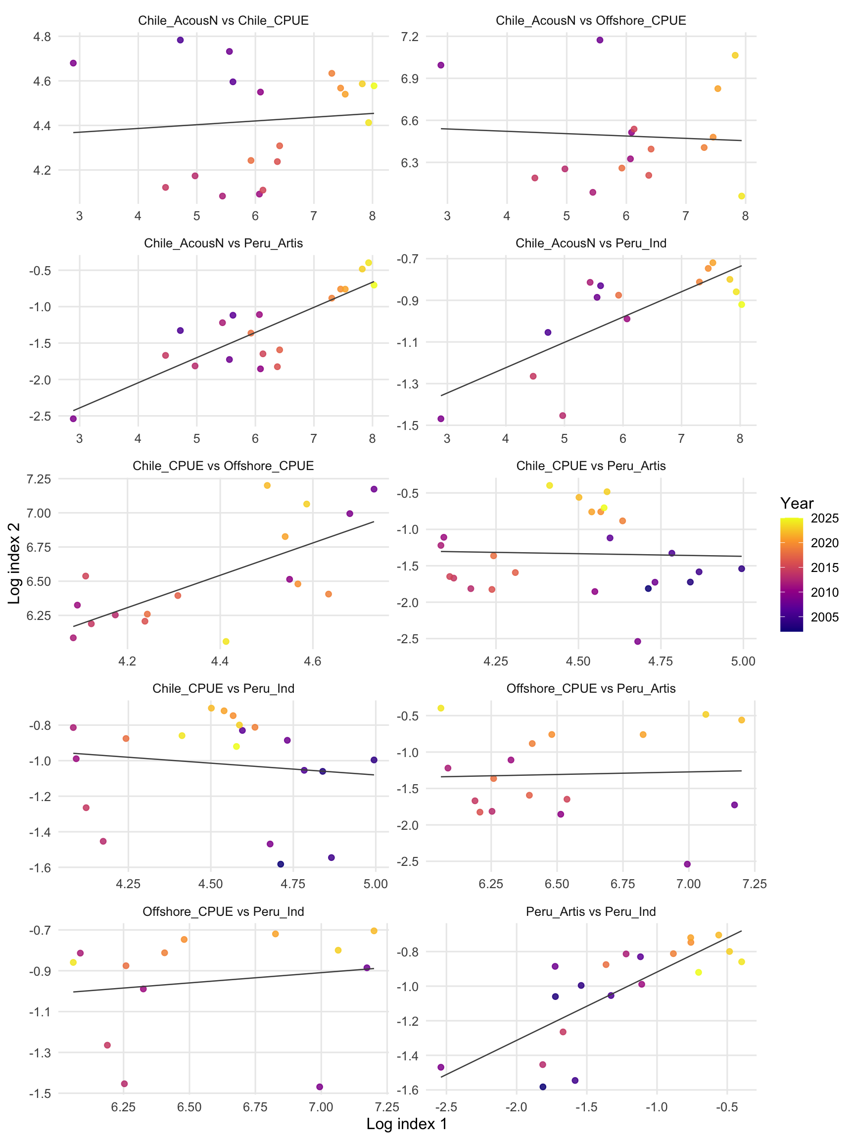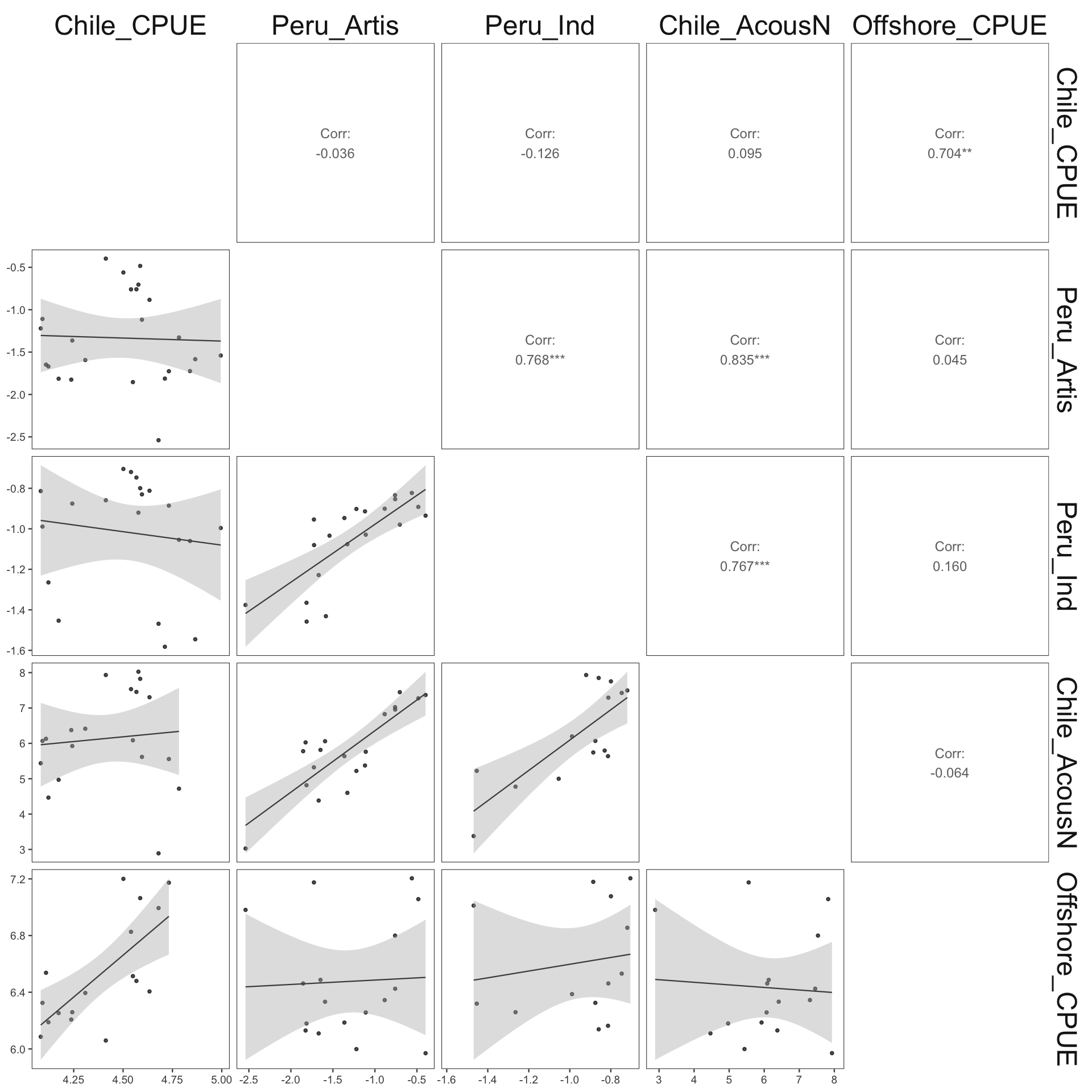@fig-correlation-pairs shows the underlying paired observations for each Pearson correlation. Each panel uses only years where both indices have positive observations, with point color indicating year and the grey line giving a simple linear fit on the log-index scale. @fig-correlation-ggpairs shows the same log-index data as a scatterplot matrix. Pearson correlations are printed in the upper triangle, while the lower triangle shows the paired observations with linear fits and uncertainty ribbons. The pairwise overlap was largest for `r overlap_summary$max_pairs`, with `r overlap_summary$max_overlap` shared years. The lowest overlap was for `r overlap_summary$min_pairs`, with `r overlap_summary$min_overlap` shared years. This difference in overlap should be considered when comparing the apparent strength of correlations across index pairs. ```{r} #| label: fig-correlation-heatmap #| fig-cap: "Pearson correlations between log observed indices after omitting Chile_AcousCS. Blue cells indicate positive correlations, red cells indicate negative correlations, and the lower triangle reports r for each pair." #| echo: false #| fig-height: 5.5 ggcorrplot( correlation_matrix, type = "lower", lab = TRUE, lab_size = 3.5, show.diag = FALSE, colors = c("#b2182b", "white", "#2166ac"), outline.color = "white", ggtheme = theme_minimal(base_size = 12) ) + labs(fill = "r") + theme( axis.text.x = element_text(angle = 45, hjust = 1), legend.position = "right" ) ``` ```{r} #| label: tbl-correlations #| tbl-cap: "Pairwise index correlations. Pearson correlations use log observed indices; Spearman correlations use observed values. Pairs with fewer than the minimum overlapping years are reported as NA." #| echo: false correlation_results |> invisible() correlation_table |> mutate( Pearson = round(Pearson, 3), Spearman = round(Spearman, 3) ) |> gt() |> tab_spanner(label = "Correlation", columns = c(Pearson, Spearman)) |> cols_label( index_1 = "index_1", index_2 = "index_2", n_overlap = "n_overlap", first_overlap = "first_overlap", last_overlap = "last_overlap" ) |> fmt_number(columns = c(Pearson, Spearman), decimals = 3) ``` ```{r} #| label: fig-correlation-pairs #| fig-cap: "Pairwise index relationships for h1_0.16, excluding Chile_AcousCS. Axes are log observed indices and points are overlapping years used in the Pearson correlations." #| echo: false #| fig-height: 12 ggplot(pair_plot_data, aes(x, y)) + geom_point(aes(color = year), size = 1.7, alpha = 0.85) + geom_smooth(method = "lm", se = FALSE, color = "grey30", linewidth = 0.45) + facet_wrap(~pair, scales = "free", ncol = 2) + scale_color_viridis_c(option = "C") + labs(x = "Log index 1", y = "Log index 2", color = "Year") + theme_report() + theme( legend.position = "right", strip.text.y = element_text(angle = 0, hjust = 0) ) ``` ```{r} #| label: fig-correlation-ggpairs #| fig-cap: "Scatterplot matrix for log observed indices. Upper panels show Pearson correlations; lower panels show paired observations with linear fits and uncertainty ribbons." #| echo: false #| fig-width: 10 #| fig-height: 10 ggpairs( pair_matrix_data, upper = list(continuous = wrap("cor", method = "pearson", use = "pairwise.complete.obs")), lower = list(continuous = ggpairs_lower_lm), diag = list(continuous = "blankDiag") ) + ggthemes::theme_few(base_size = 9) + theme(strip.text = element_text(size = 18)) ``` ## Patterns in model fit residuals The observation correlations above describe whether index observations move together. A complementary diagnostic is to compare model fit residuals, because shared residual patterns indicate years where indices contain similar information after the `h1_0.16` model fit has already explained the common stock trend. This is more directly related to availability trade-offs among indices: two indices with strongly correlated residuals are likely to add less independent information than two indices whose residuals differ. 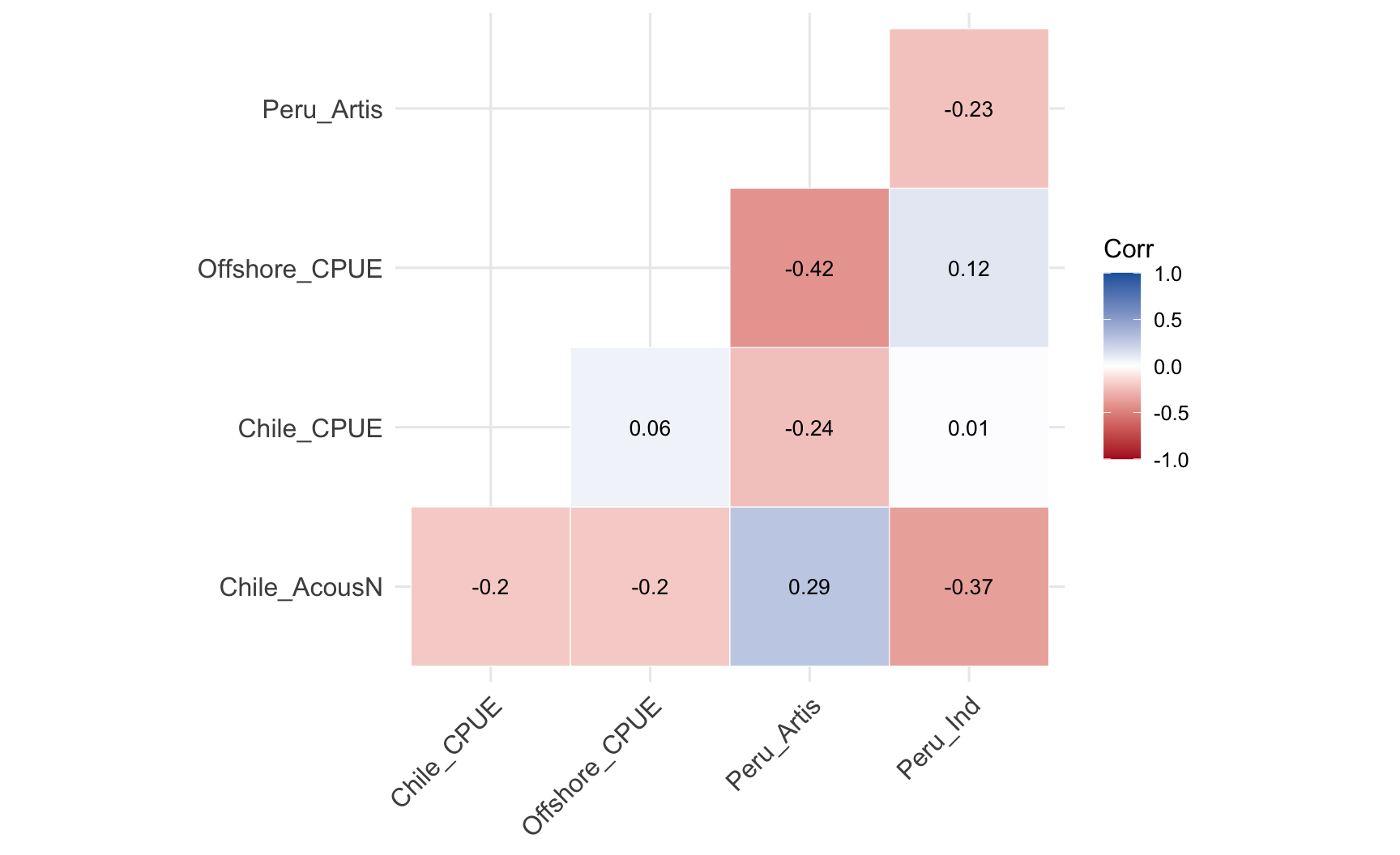@tbl-residual-summary gives the retained residual coverage by index for `h1_0.16` and `h2_0.16`. Residuals are the standardized index-fit residuals reported in the JJM `Obs_Survey_*` output, after omitting `Chile_AcousCS` and dropping `Chile_AcousN` observations before 2006. @fig-h1-residual-correlation-heatmap shows the Pearson correlations among residuals for the one-stock hypothesis; @fig-h2-residual-correlation-heatmap shows the same diagnostic for the two-stock hypothesis. ```{r} #| label: tbl-residual-summary #| tbl-cap: "Model fit residual coverage by model and index. Residuals are standardized index-fit residuals from the JJM Obs_Survey output." #| echo: false residual_summary |> arrange(model, index) |> gt() |> fmt_number(columns = c(mean_residual, sd_residual), decimals = 3) ``` ```{r} #| label: fig-h1-residual-correlation-heatmap #| fig-cap: "Pearson correlations between standardized model fit residuals for retained indices in h1_0.16. Blue cells indicate positive residual correlations and red cells indicate negative residual correlations." #| echo: false #| fig-height: 5.5 ggcorrplot( h1_residual_correlation_matrix, type = "lower", lab = TRUE, lab_size = 3.5, show.diag = FALSE, colors = c("#b2182b", "white", "#2166ac"), outline.color = "white", ggtheme = theme_minimal(base_size = 12) ) + labs(fill = "r") + theme( axis.text.x = element_text(angle = 45, hjust = 1), legend.position = "right" ) ``` For `h2_0.16`, the residual correlations span the two-stock model structure. The `Peru_Artis` and `Peru_Ind` residuals come from stock 2, while `Chile_AcousN`, `Chile_CPUE`, and `Offshore_CPUE` come from stock 1. Within stock 2, the residual correlation between `Peru_Artis` and `Peru_Ind` was `r sprintf("%.2f", h2_stock2_residual_correlation)` across `r nrow(h2_stock2_residual_pair)` overlapping years (`r min(h2_stock2_residual_pair$year)`-`r max(h2_stock2_residual_pair$year)`). Pairs with strong positive residual correlations indicate indices that still tend to be high or low together after fitting their stock-specific trends; pairs closer to zero or negative values indicate more distinct residual information and may be more informative for availability trade-offs. Cross-stock residual correlations should therefore be read as comparisons between independently fitted stock components rather than as residuals from a single shared abundance trajectory. ```{r} #| label: fig-h2-residual-correlation-heatmap #| fig-cap: "Pearson correlations between standardized model fit residuals for retained indices in h2_0.16. Blue cells indicate positive residual correlations and red cells indicate negative residual correlations." #| echo: false #| fig-height: 5.5 ggcorrplot( h2_residual_correlation_matrix, type = "lower", lab = TRUE, lab_size = 3.5, show.diag = FALSE, colors = c("#b2182b", "white", "#2166ac"), outline.color = "white", ggtheme = theme_minimal(base_size = 12) ) + labs(fill = "r") + theme( axis.text.x = element_text(angle = 45, hjust = 1), legend.position = "right" ) ``` ## Index ROC/AUC 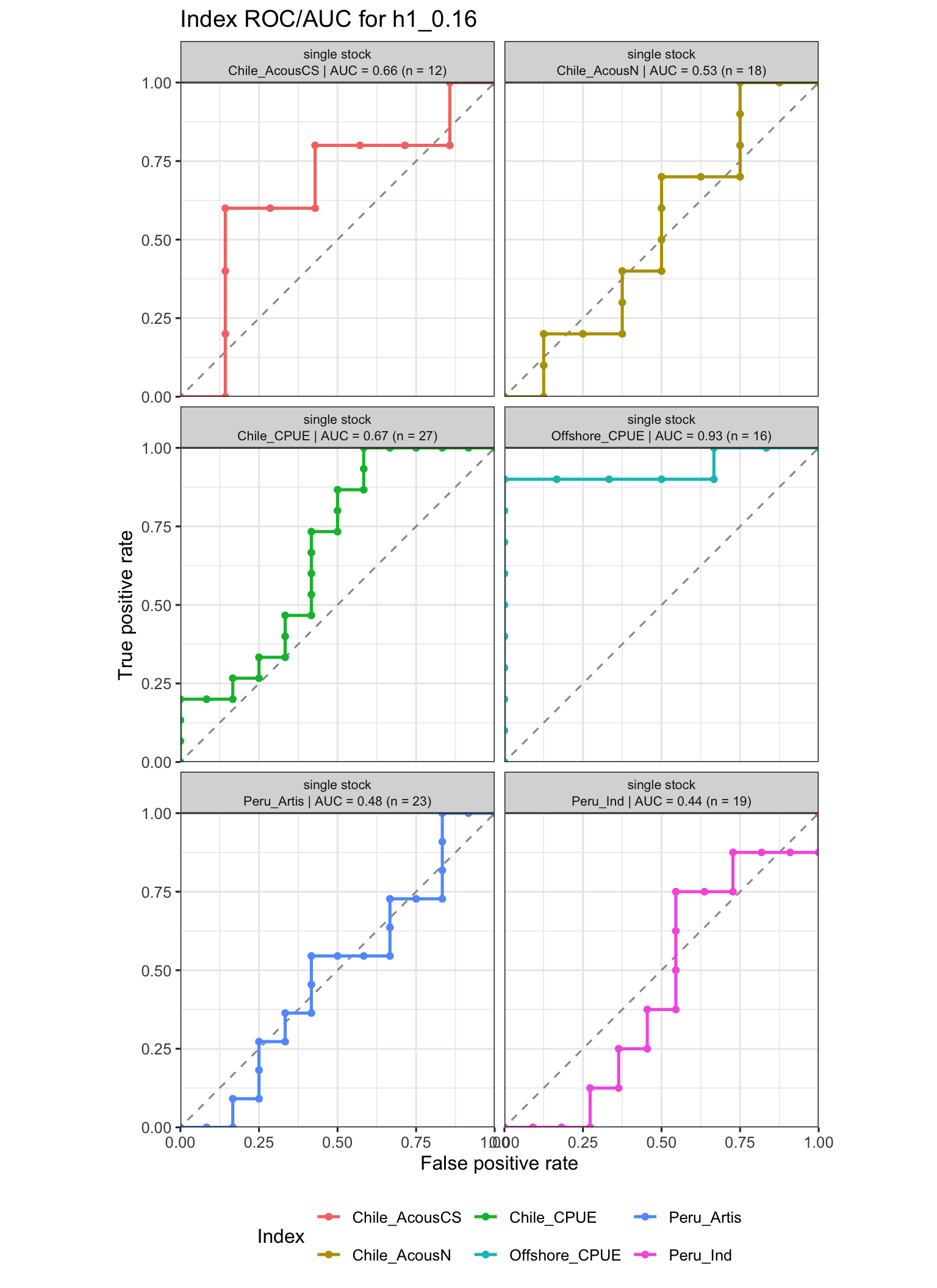The ROC/AUC diagnostics below are loaded from the `jmMSE` output file `output/index_auc_h1_h2_0.16.rda`. They compare annual index changes against annual changes in model-estimated SSB. For each index, the score is $\log(I_y / I_{y-1})$ and the truth is whether $SSB_y > SSB_{y-1}$. For `h1_0.16`, each index is compared with the single-stock SSB trajectory. For `h2_0.16`, each index is compared with the SSB trajectory for the stock-specific output block in which the index appears. The `Chile_AcousN` ROC diagnostic uses only observations after 2005, following the implementation in `jmMSE/output_auc_peru_cpue.R`. @fig-h1-index-roc shows the h1 single-stock ROC diagnostics. Curves above the one-to-one dashed line indicate that positive index changes tend to coincide with years when model-estimated SSB increased; AUC values closer to one indicate stronger discrimination. 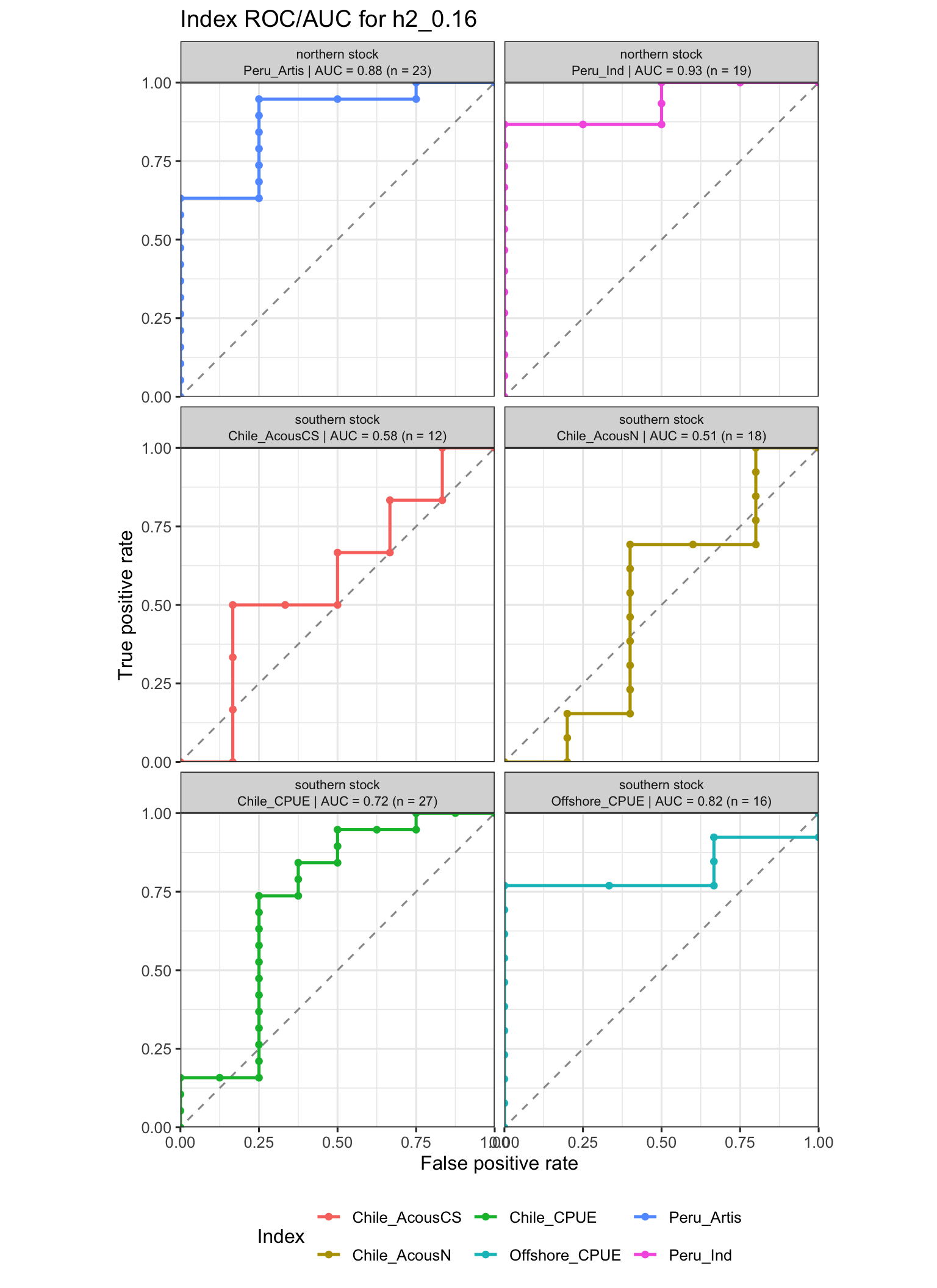@fig-h2-index-roc applies the same diagnostic to the h2 stock-specific outputs. The southern-stock indices and northern-stock indices are evaluated against their corresponding stock-specific SSB changes, so these panels should not be interpreted as a single pooled-stock diagnostic. @tbl-index-roc-auc summarizes the AUC and number of annual index changes used in each ROC curve from @fig-h1-index-roc and @fig-h2-index-roc. ```{r} #| label: fig-h1-index-roc #| fig-cap: "Receiver Operating Characteristic (ROC) curves for abundance indices as indicators of changes in spawning stock biomass (SSB) in h1_0.16. Chile_AcousN uses only observations after 2005." #| echo: false #| fig-width: 8 #| fig-height: 11 ggplot(h1_index_roc, aes(x = FPR, y = TPR, color = index)) + geom_abline(slope = 1, intercept = 0, linetype = "dashed", color = "grey60") + geom_step(linewidth = 0.9, direction = "hv") + geom_point(size = 1.5) + facet_wrap(~facet, ncol = 2) + coord_equal(xlim = c(0, 1), ylim = c(0, 1), expand = FALSE) + scale_x_continuous(breaks = seq(0, 1, by = 0.25)) + scale_y_continuous(breaks = seq(0, 1, by = 0.25)) + labs( title = "Index ROC/AUC for h1_0.16", x = "False positive rate", y = "True positive rate", color = "Index" ) + theme_bw(base_size = 12) + theme( legend.position = "bottom", strip.text = element_text(size = 8, lineheight = 1.05, margin = margin(4, 4, 4, 4)), strip.background = element_rect(fill = "grey85", color = "grey20") ) ``` ```{r} #| label: fig-h2-index-roc #| fig-cap: "Receiver Operating Characteristic (ROC) curves for abundance indices as indicators of changes in stock-specific spawning stock biomass (SSB) in h2_0.16. Chile_AcousN uses only observations after 2005." #| echo: false #| fig-width: 8 #| fig-height: 11 ggplot(h2_index_roc, aes(x = FPR, y = TPR, color = index)) + geom_abline(slope = 1, intercept = 0, linetype = "dashed", color = "grey60") + geom_step(linewidth = 0.9, direction = "hv") + geom_point(size = 1.5) + facet_wrap(~facet, ncol = 2) + coord_equal(xlim = c(0, 1), ylim = c(0, 1), expand = FALSE) + scale_x_continuous(breaks = seq(0, 1, by = 0.25)) + scale_y_continuous(breaks = seq(0, 1, by = 0.25)) + labs( title = "Index ROC/AUC for h2_0.16", x = "False positive rate", y = "True positive rate", color = "Index" ) + theme_bw(base_size = 12) + theme( legend.position = "bottom", strip.text = element_text(size = 8, lineheight = 1.05, margin = margin(4, 4, 4, 4)), strip.background = element_rect(fill = "grey85", color = "grey20") ) ``` ```{r} #| label: tbl-index-roc-auc #| tbl-cap: "Index ROC/AUC summaries for h1_0.16 and h2_0.16. The truth is annual SSB direction and the score is the annual log index ratio." #| echo: false index_roc_summary |> mutate(auc = round(auc, 3)) |> arrange(model, stock, desc(auc)) |> gt() |> fmt_number(columns = auc, decimals = 3) ``` ## Summary @tbl-strongest-correlations extracts the largest positive and most negative Pearson correlations from the correlation table. This is a compact way to identify the index pairs with the strongest agreement and strongest disagreement after accounting for the available overlapping years. This evaluation shows that, for the two-stock hypotheses, the nominal CPUE indices for Peru generally track stock trends. Those same indices perform relatively poorer under the single-stock hypothesis. For the single-stock case, the offshore CPUE and Chilean CPUE indices appear to perform better. These conclusions are broadly consistent between the pairwise index comparisons and the ROC/AUC evaluations. 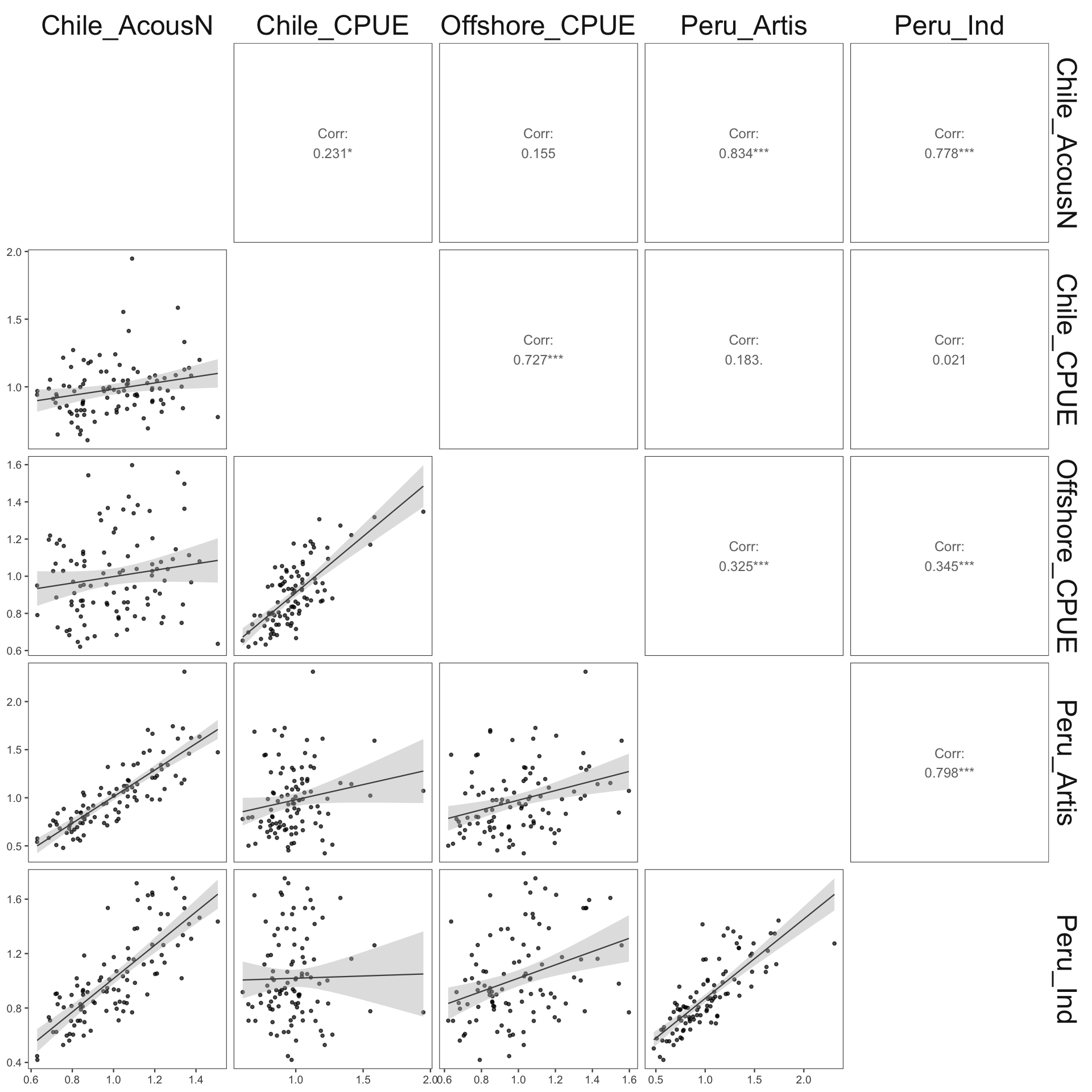@tbl-index-covariance-matrix reports the covariance matrix used to simulate the multivariate index draws in long form. @fig-index-covariance-draws uses that estimated correlation structure among the retained index series to simulate 100 multivariate draws. The simulation uses the Pearson correlations among log observed indices for `Chile_AcousN`, `Chile_CPUE`, `Offshore_CPUE`, `Peru_Artis`, and `Peru_Ind`; the diagonal uncertainty is set to 20% CV for all indices except the two Peruvian CPUE series, which use 30% CV. 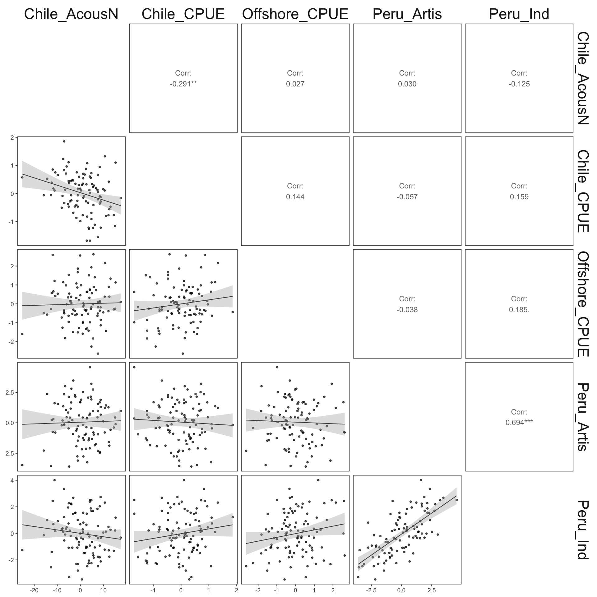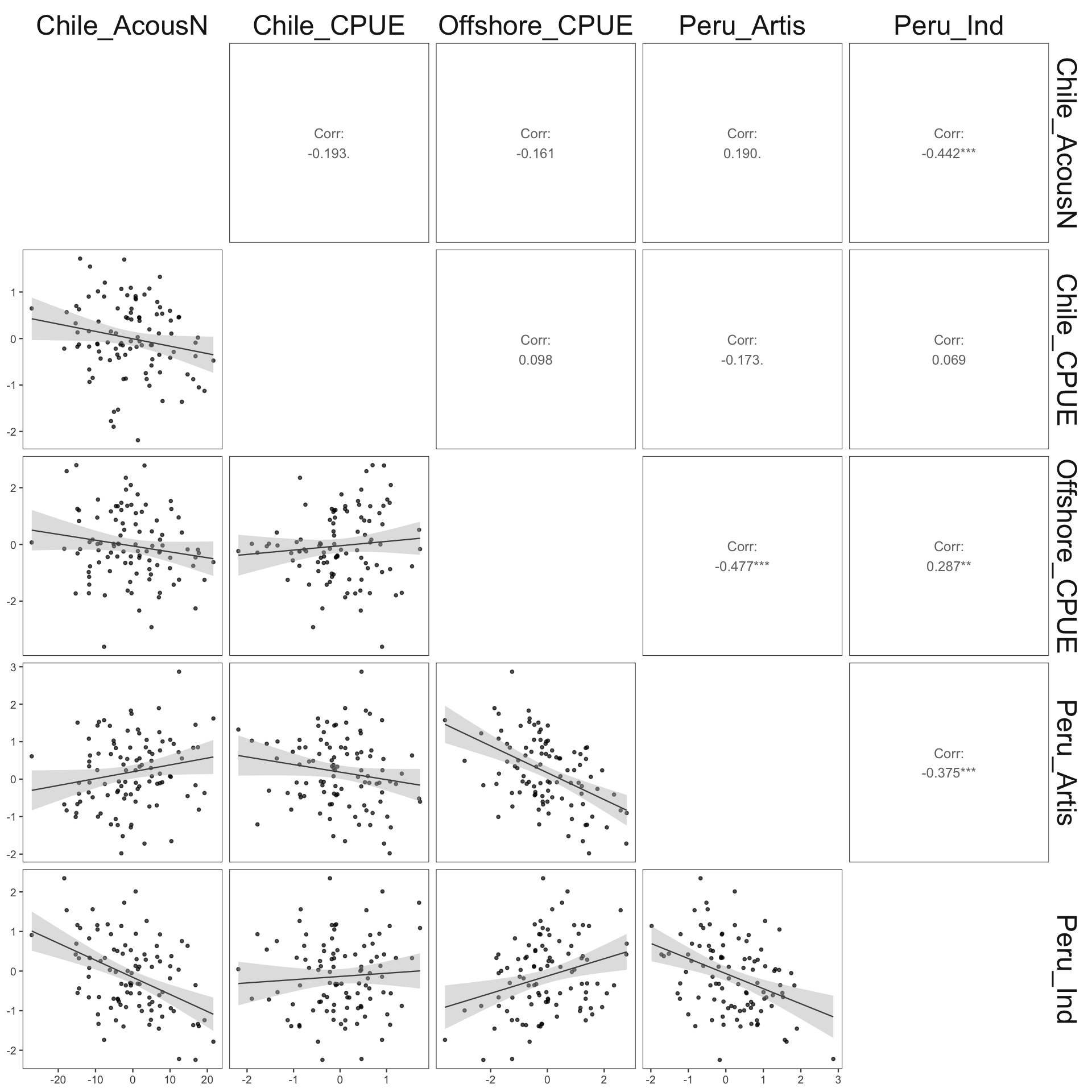@tbl-h1-residual-covariance-matrix and @tbl-h2-residual-covariance-matrix report the fitted-residual covariance structures used for residual-based simulations. @fig-h1-residual-covariance-draws and @fig-h2-residual-covariance-draws use the residual covariance among retained indices for `h1_0.16` and `h2_0.16`, respectively. In these residual-based simulations, the diagonal is not externally specified; it is the empirical variance of the model fit residuals for each index. ```{r} #| label: tbl-strongest-correlations #| tbl-cap: "Strongest positive and negative contrasts. Based on Pearson correlations of log-observed indices." #| echo: false correlation_results |> filter(method == "Pearson", scale == "log observed", !is.na(correlation)) |> group_by(model) |> slice_max(correlation, n = 3, with_ties = FALSE) |> bind_rows( correlation_results |> filter(method == "Pearson", scale == "log observed", !is.na(correlation)) |> group_by(model) |> slice_min(correlation, n = 3, with_ties = FALSE) ) |> ungroup() |> distinct(model, index_1, index_2, .keep_all = TRUE) |> arrange(model, desc(correlation)) |> select(index_1, index_2, n_overlap, first_overlap, last_overlap, correlation) |> mutate(correlation = round(correlation, 3)) |> gt() |> fmt_number(columns = correlation, decimals = 3) ``` ```{r} #| label: tbl-index-covariance-matrix #| tbl-cap: "Long-form covariance matrix used to generate the simulated multivariate index draws. Covariances are on the log-index multiplier scale after converting specified CVs to log-scale standard deviations." #| echo: false covariance_matrix_long |> mutate( cv_1 = sprintf("%.0f%%", 100 * cv_1), cv_2 = sprintf("%.0f%%", 100 * cv_2) ) |> gt() |> cols_label( index_1 = "index_1", index_2 = "index_2", cv_1 = "cv_1", cv_2 = "cv_2", correlation = "correlation", covariance = "covariance" ) |> fmt_number(columns = c(correlation, covariance), decimals = 4) ``` ```{r} #| label: fig-index-covariance-draws #| fig-cap: "Simulated multivariate index draws using the estimated correlation structure among retained indices. Diagonal uncertainty assumes 20% CV except Peru_Artis and Peru_Ind, which use 30% CV." #| echo: false #| fig-width: 10 #| fig-height: 10 ggpairs( index_covariance_draws, upper = list(continuous = wrap("cor", method = "pearson")), lower = list(continuous = ggpairs_lower_lm), diag = list(continuous = "blankDiag") ) + ggthemes::theme_few(base_size = 9) + theme(strip.text = element_text(size = 18)) ``` ```{r} #| label: tbl-h1-residual-covariance-matrix #| tbl-cap: "Long-form covariance matrix used to generate simulated residual draws for h1_0.16. Covariances are computed from standardized index-fit residuals." #| echo: false h1_residual_covariance_long |> gt() |> fmt_number(columns = c(correlation, covariance), decimals = 4) ``` ```{r} #| label: fig-h1-residual-covariance-draws #| fig-cap: "Simulated multivariate residual draws for h1_0.16 using the estimated covariance structure among retained index fit residuals. Diagonal uncertainty is the empirical residual variance for each index." #| echo: false #| fig-width: 10 #| fig-height: 10 ggpairs( h1_residual_covariance_draws, upper = list(continuous = wrap("cor", method = "pearson")), lower = list(continuous = ggpairs_lower_lm), diag = list(continuous = "blankDiag") ) + ggthemes::theme_few(base_size = 9) + theme(strip.text = element_text(size = 18)) ``` ```{r} #| label: tbl-h2-residual-covariance-matrix #| tbl-cap: "Long-form covariance matrix used to generate simulated residual draws for h2_0.16. Covariances are computed from standardized index-fit residuals." #| echo: false h2_residual_covariance_long |> gt() |> fmt_number(columns = c(correlation, covariance), decimals = 4) ``` ```{r} #| label: fig-h2-residual-covariance-draws #| fig-cap: "Simulated multivariate residual draws for h2_0.16 using the estimated covariance structure among retained index fit residuals. Diagonal uncertainty is the empirical residual variance for each index." #| echo: false #| fig-width: 10 #| fig-height: 10 ggpairs( h2_residual_covariance_draws, upper = list(continuous = wrap("cor", method = "pearson")), lower = list(continuous = ggpairs_lower_lm), diag = list(continuous = "blankDiag") ) + ggthemes::theme_few(base_size = 9) + theme(strip.text = element_text(size = 18)) ```

SPRFMO