
flowchart LR
  A["boot/initial/data/<year>/<model><br/>JJM .ctl and .dat inputs"] --> B["data_condition.R<br/>models table"]
  B --> C["conditionJJOM() in utilities.R"]
  C --> D["FLjjm::exejjms()<br/>FLjjm::calljjms()"]
  D --> E["jjms ADMB run"]
  E --> F["data/cond_<short>_<model>_<opt>_<set>/"]
  F --> G["adnuts::sample_nuts()<br/>posterior samples"]
  G --> H["mcout_<model>.rds<br/>mceval.rep.gz"]
  F --> I["data_load.R"]
  I --> J["constructJJOM() in utilities.R"]
  J --> K["FLjjm::readFLomjjm()<br/>FLjjm::readFLoemjjm()"]
  K --> L["OM bundle<br/>om + oem + iem + srdevs + unfishedSSB"]
  L --> M["data/<short>_<model>_<opt>.rds"]
Jack mackerel MSE workflow
SPRFMO
South Pacific Regional Fisheries Management Organisation
Jack Mackerel Working Group
Jack mackerel MSE workflow
1 Purpose
This note is a working map of the software layers used in the jack mackerel management strategy evaluation (MSE) workflow. It is intended to explain how operating models (OMs) are created from JJM assessment configurations, how management procedures (MPs) are specified in jmMSE, and how candidate MPs are tested against performance metrics.
The short version is:
- JJM is the assessment engine.
jjmRreads and writes JJM input and output files.FLjjmruns JJM and converts JJM output into FLR/mse objects.jmMSEdefines the OM set, candidate MPs, simulations, tuning, diagnostics, and reports.mse,msemodules,FLCore,FLFishery, andFLasherprovide the simulation object classes and MP machinery.
2 Package Roles
| Layer | Main responsibility | Typical objects or files |
|---|---|---|
| JJM | Compiled ADMB stock assessment model for Chilean jack mackerel | jjms, .ctl, .dat, .rep, .std, .par, For_R_*.rep |
jjmR |
Low-level R input/output layer for JJM | writeJJM(), readJJM(), jjm.output |
FLjjm |
Adapter between JJM and FLR/mse | readFLomjjm(), readFLSjjm(), readFLIsjjm(), cjm.oem(), cjm.iem(), jjms.sa(), statistics |
| FLR/mse stack | Generic MSE classes, projection, and MP execution | FLStock, FLStocks, FLIndex, FLIndices, FLombf, FLoem, FLiem, mpCtrl(), mseCtrl(), mp() |
jmMSE |
Project-specific workflow and candidate MP testing | data_condition.R, data_load.R, model_*.R, utilities.R, reports, tests |
3 Overall Flow
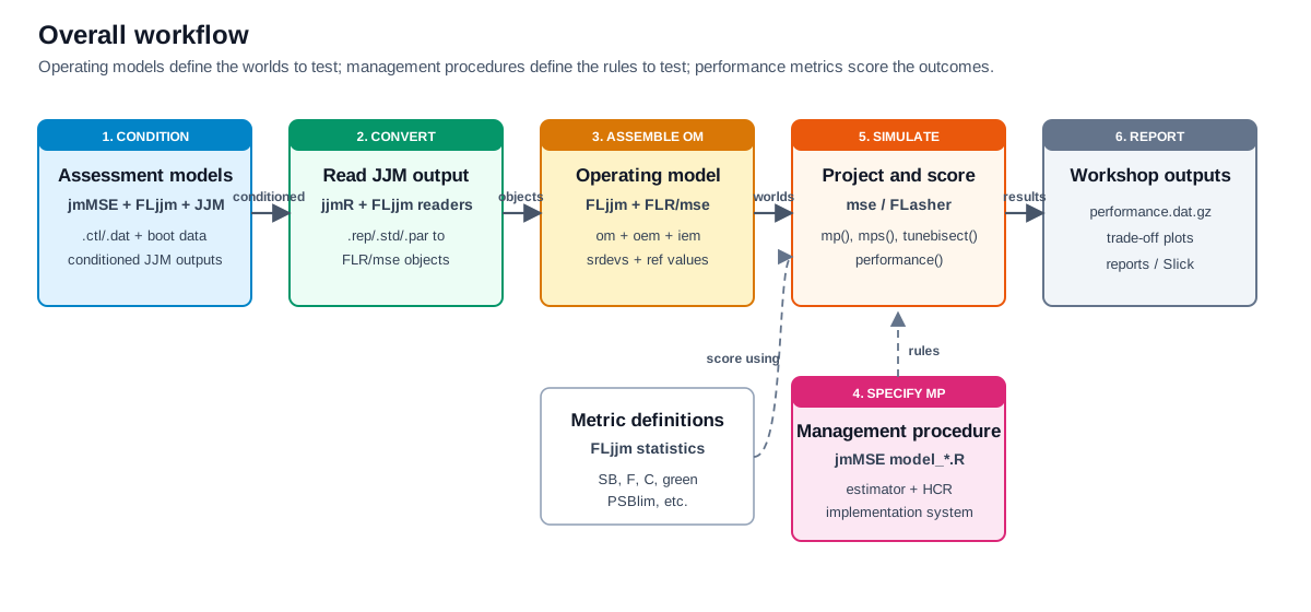
4 Operating Model Construction
In jmMSE, the OM set is currently defined as a table of model configurations in data_condition.R. Each row identifies a JJM model, source year, option, robustness or reference status, working directory, and output file name.
The important distinction is that JJM defines the assessment-conditioned biological and fishery dynamics, while FLjjm converts those results into FLR/mse objects that can be projected under candidate MPs.
Typical OM bundle fields are:
| Field | Meaning |
|---|---|
om |
The operating model, usually an FLombf object containing biology, fisheries, reference points, and projection method. |
oem |
The observation error model, usually a FLoem object with simulated index observations. |
iem |
The implementation error model, usually an FLiem object controlling how TAC or catch advice is implemented across fisheries. |
srdevs |
Recruitment-deviation scenarios derived from historical OM recruitment deviances. |
unfishedSSB |
Reference unfished biomass metric generated for comparison or derived performance metrics. |
5 Management Procedure Specification
Candidate MPs are specified through mse::mpCtrl() as three linked modules:
| MP component | Role | Examples in jmMSE |
|---|---|---|
est |
Estimator or assessment module used inside the MP | shortcut.sa, cpue.ind, spict.sa, perfect.sa, jjms.sa |
hcr |
Harvest control rule that turns estimated status into advice | buffer.hcr, hockeystick.hcr, fixedC.hcr |
isys |
Implementation system that distributes advice into fisheries or stocks | split.is, usually with catch_props(om)$last5 |
Typical structure:
ctrl <- mpCtrl(
  est = mseCtrl(
    method = shortcut.sa,
    args = list(metric = "depletion", devs = metdevs, B0 = refpts(om)$SB0)
  ),
  hcr = mseCtrl(
    method = hockeystick.hcr,
    args = list(
      lim = 0.10, trigger = 0.40, metric = "depletion",
      target = mean(refpts(om)$MSY), output = "catch"
    )
  ),
  isys = mseCtrl(
    method = split.is,
    args = list(split = catch_props(om)$last5)
  )
)
Then the MP is run against an OM:
run <- mp(
  om,
  oem = oem,
  iem = iem,
  ctrl = ctrl,
  args = list(iy = 2025, fy = 2050)
)
6 Testing Against Performance Metrics
Performance metrics are mostly evaluated through mse::performance(), using the statistics dataset loaded from FLjjm in config.R.
flowchart TD
  OM["Operating model<br/>om + oem + iem"] --> MP["Candidate MP<br/>est + hcr + isys"]
  MP --> SIM["mp(), mps(), or tunebisect()<br/>future projections by iteration"]
  SIM --> TRACK["simulation output and tracking<br/>stock, catch, decisions, estimates"]
  STATS["FLjjm statistics<br/>C, F, SB, SBMSY, green, PSBlim, etc."] --> PERF["performance()"]
  TRACK --> PERF
  PERF --> TABLE["performance table<br/>statistic x year x MP x OM"]
  TABLE --> TUNE["tuning decisions<br/>e.g., target giving P(green) = 0.6"]
  TABLE --> REPORT["trade-off plots<br/>tables, reports, Slick app"]
Common calls in the local workflow are:
performance(run, statistics = statistics["green"], years = ty)

tuned <- tunebisect(
  om,
  oem = oem,
  iem = iem,
  control = ctrl,
  statistic = statistics["green"],
  years = ty,
  prob = 0.6
)

runs <- FLmses(list(tune06 = tuned), statistics = statistics)
7 Local Code Map
| Purpose | Local file |
|---|---|
Load core packages and FLjjm statistics |
jmMSE/config.R |
| Define the conditioned JJM model grid | jmMSE/data_condition.R |
| Run JJM and ADNUTS for conditioned OMs | jmMSE/utilities.R, conditionJJOM() |
| Convert conditioned JJM runs into OM bundles | jmMSE/data_load.R, constructJJOM() |
| Read FLR objects from JJM output | FLjjm/R/read.R |
Execute bundled jjms model |
FLjjm/R/run.R |
| CJM-specific OEM/IEM and JJM assessment modules | FLjjm/R/mse.R |
| Shortcut MP examples | jmMSE/model_shortcut.R |
| Fixed-catch MP examples | jmMSE/model_fixed.R |
| SPiCT MP examples and helper functions | jmMSE/model_spict.R, jmMSE/utilities.R |
| Tests and diagnostics | jmMSE/tests/ |
8 Mental Model
The workflow is easiest to read as a data transformation:
flowchart LR
  A["Assessment inputs<br/>JJM .ctl/.dat"] --> B["Conditioned JJM run"]
  B --> C["FLjjm conversion"]
  C --> D["MSE operating model"]
  D --> E["Candidate MP"]
  E --> F["Future simulation"]
  F --> G["Performance metrics"]
  G --> H["Trade-off and robustness decisions"]
The OM describes the world being tested. The MP describes the rule being tested. The performance metrics describe how that rule behaves across simulated futures and robustness scenarios.