---
title: "SCW17/Paper-07 Projection evaluations"
subtitle: "Forward projection scenarios and selectivity sensitivity from jmMSE"
date: today
format:
html:
output-file: "SCW17-Paper-07-Projection-evaluations.html"
toc: true
toc-depth: 3
number-sections: true
theme: cosmo
code-fold: true
code-summary: "Show code"
code-tools: true
lightbox: true
execute:
echo: true
warning: false
message: false
params:
jmMSE_path: "../../jmMSE"
---
```{r}
#| label: setup
#| include: false
library(ggplot2)
library(ggthemes)
library(data.table)
library(knitr)
library(FLCore)
library(mse)
jmMSE_path <- params$jmMSE_path
cache_file <- file.path(jmMSE_path, "report", "projections", "cache.rda")
if(!file.exists(cache_file)) {
stop("Projection cache not found at ", cache_file,
". Run source('run_projections.R') in the jmMSE repository before ",
"rendering this report.")
}
load(cache_file)
load(file.path(jmMSE_path, "data", "models.rda"))
fmt_num <- function(x, digits=0) {
format(round(x, digits), big.mark=",", trim=TRUE, scientific=FALSE)
}
fmt_value <- function(x) {
if(is.character(x)) x else fmt_num(x, digits=3)
}
scenario_tbl <- do.call(rbind, lapply(names(SCENARIOS), function(nm) {
desc <- SCENARIOS[[nm]]$description
if(is.null(desc)) desc <- ""
data.frame(
scenario = nm,
control_quantity = SCENARIOS[[nm]]$quant,
target = fmt_value(SCENARIOS[[nm]]$value),
description = desc,
stringsAsFactors = FALSE
)
}))
refpt_tbl <- data.frame(
stock = names(sbmsy_ref),
SBMSY_t = fmt_num(unname(sbmsy_ref), 0),
FMSY = fmt_num(unname(fmsy_ref), 3),
stringsAsFactors = FALSE
)
current_tbl <- as.data.frame(state_dt)
current_tbl$ssb <- fmt_num(current_tbl$ssb)
current_tbl$catch <- fmt_num(current_tbl$catch)
current_tbl$sbmsy <- fmt_num(current_tbl$sbmsy)
current_tbl$f <- fmt_num(current_tbl$f, 3)
current_tbl$fmsy <- fmt_num(current_tbl$fmsy, 3)
current_tbl$ssb_sbmsy <- fmt_num(current_tbl$ssb_sbmsy, 2)
fleet_split_tbl <- NULL
if(exists("cprop")) {
fleet_split_tbl <- data.frame(
fleet = names(cprop),
share = fmt_num(100 * unname(cprop), 1),
stringsAsFactors = FALSE
)
}
block_tbl <- do.call(rbind, lapply(names(SELEX_BLOCKS), function(nm) {
yrs <- SELEX_BLOCKS[[nm]]
data.frame(
block = nm,
years = paste(min(yrs), max(yrs), sep="-"),
stringsAsFactors = FALSE
)
}))
FBAR_MAX <- 0.8
filter_note <- paste("Results with Fbar greater than", FBAR_MAX, "are excluded.")
scenario_caption <- function() {
ref_txt <- paste(mapply(function(s, sbm, fms)
sprintf("%s: SBMSY = %s t, FMSY = %s", s,
format(round(sbm), big.mark=","), round(fms, 3)),
names(sbmsy_ref), sbmsy_ref, fmsy_ref), collapse=" | ")
paste("Forward projections under the future fishing-pattern scenarios.",
ref_txt, paste0("Projections: ", INIT_YEAR + 1, "-", FINAL_YEAR),
filter_note)
}
sensitivity_caption <- function(prefix) {
ref_txt <- paste(mapply(function(s, sbm, fms)
sprintf("%s: SBMSY = %s t, FMSY = %s", s,
format(round(sbm), big.mark=","), round(fms, 3)),
names(sbmsy_ref), sbmsy_ref, fmsy_ref), collapse=" | ")
paste(prefix, ref_txt, filter_note)
}
median_fbar_exclusions <- function(dat, group_col, fbar_max=FBAR_MAX) {
dat <- as.data.table(dat)
if(!"Fbar" %in% dat$metric)
return(data.table())
dat[metric == "Fbar",
.(max_median_fbar=max(value, na.rm=TRUE)),
by=c(group_col, "stock")][max_median_fbar > fbar_max]
}
drop_group_stock <- function(dat, excluded, group_col) {
dat <- as.data.table(copy(dat))
if(nrow(excluded) == 0)
return(dat)
dat[!excluded[, .SD, .SDcols=c(group_col, "stock")],
on=c(group_col, "stock")]
}
drop_fbar_iterations <- function(dat, fbar_max_dt, group_col, fbar_max=FBAR_MAX) {
dat <- as.data.table(copy(dat))
if(is.null(fbar_max_dt) || nrow(fbar_max_dt) == 0 || !"iter" %in% names(dat))
return(dat)
excluded <- as.data.table(fbar_max_dt)[max_fbar > fbar_max,
.SD, .SDcols=c(group_col, "stock", "iter")]
if(nrow(excluded) == 0)
return(dat)
dat[!excluded, on=c(group_col, "stock", "iter")]
}
report_theme <- function(base_size=16) {
ggthemes::theme_few(base_size=base_size) +
theme(
plot.title=element_text(size=base_size + 4, face="bold"),
plot.subtitle=element_text(size=base_size + 1),
axis.title=element_text(size=base_size + 1),
axis.text=element_text(size=base_size),
strip.text=element_text(size=base_size, face="bold"),
legend.title=element_text(size=base_size),
legend.text=element_text(size=base_size - 1),
legend.position="bottom"
)
}
zero_y_scale <- function(...) {
scale_y_continuous(limits=c(0, NA), expand=expansion(mult=c(0, 0.05)), ...)
}
scale_colour_cycling <- function(x, ...) {
pal <- c("#cc79a7", "#009e73", "#e69f00", "#56b4e9", "#999999",
"#f0e442", "#0072b2", "#d55e00")
lvls <- if(is.factor(x)) levels(x) else unique(as.character(x))
scale_colour_manual(values=setNames(pal[(seq_along(lvls) - 1L) %% length(pal) + 1L], lvls), ...)
}
metric_panels <- function(dat, ref_lines=NULL) {
metric_levels <- c("SSB (t)", "Fbar", "Catch (kt)", "F[a=1-12]",
"F[a=3-8]", "F[N-wtd]", "HR")
dat <- as.data.table(copy(dat))
if("metric" %in% names(dat)) {
dat[metric == "Catch (t)", metric := "Catch (kt)"]
m_present <- unique(as.character(dat$metric))
m_levels <- c(intersect(metric_levels, m_present), setdiff(m_present, metric_levels))
dat[, metric := factor(as.character(metric), levels=m_levels)]
}
if(!is.null(ref_lines)) {
ref_lines <- as.data.table(copy(ref_lines))
if("metric" %in% names(ref_lines))
ref_lines[, metric := factor(as.character(metric), levels=levels(dat$metric))]
}
multi_stock <- "stock" %in% names(dat) && length(unique(dat$stock)) > 1
if(multi_stock) {
s_lvls <- as.character(unique(dat$stock))
m_lvls <- as.character(unique(dat$metric))
panel_lvls <- as.vector(outer(s_lvls, m_lvls, function(s, m) paste(m, s, sep="\n")))
dat[, panel := factor(paste(metric, stock, sep="\n"), levels=panel_lvls)]
if(!is.null(ref_lines))
ref_lines[, panel := factor(paste(metric, stock, sep="\n"), levels=panel_lvls)]
list(dat=dat, ref_lines=ref_lines, multi_stock=TRUE, ncol=length(s_lvls))
} else {
list(dat=dat, ref_lines=ref_lines, multi_stock=FALSE, ncol=1)
}
}
plot_qmd_selectivity <- function(selex_ts_dt, ref_om=NULL) {
title <- if(!is.null(ref_om))
paste("Catch selectivity at age by fishery -", ref_om)
else "Catch selectivity at age by fishery"
multi_stock <- "stock" %in% names(selex_ts_dt) && length(unique(selex_ts_dt$stock)) > 1
ggplot(selex_ts_dt, aes(x=age, y=sel, group=year, colour=year)) +
geom_line(linewidth=0.7, alpha=0.85) +
scale_colour_viridis_c(name="Year") +
zero_y_scale() +
{ if(multi_stock) facet_grid(stock ~ fishery) else facet_wrap(~fishery, ncol=2) } +
labs(title=title, x="Age", y="Selectivity") +
report_theme() +
theme(legend.position="right")
}
plot_qmd_exploitation <- function(mets_dt, worms_dt=NULL, init_year, n_iter=NULL, ref_om=NULL) {
title <- if(!is.null(ref_om))
paste("Exploitation metrics -", ref_om, "(historical)")
else "Exploitation metrics (historical)"
sub <- if(!is.null(n_iter)) paste("80% interval across", n_iter, "iterations")
else "80% interval across iterations"
if(!is.null(worms_dt) && nrow(worms_dt) > 0)
sub <- paste0(sub, " | colored lines: ", length(unique(worms_dt$iter)), " MCMC draws")
sum_dt <- as.data.table(mets_dt)[year <= init_year,
.(q10=quantile(value, 0.10, na.rm=TRUE),
q50=median(value, na.rm=TRUE),
q90=quantile(value, 0.90, na.rm=TRUE)),
by=.(stock, metric, year)]
panel <- metric_panels(sum_dt)
sum_dt <- panel$dat
if(!is.null(worms_dt) && nrow(worms_dt) > 0) {
worms_dt <- metric_panels(as.data.table(worms_dt)[year <= init_year])$dat
worm_lvls <- sort(unique(worms_dt$iter))
worm_cols <- setNames(grDevices::hcl.colors(length(worm_lvls), "Viridis"),
worm_lvls)
worms_dt[, worm_col := worm_cols[as.character(iter)]]
}
p <- ggplot(sum_dt, aes(x=year)) +
geom_ribbon(aes(ymin=q10, ymax=q90), fill="#d55e00", alpha=0.18, colour=NA) +
{ if(!is.null(worms_dt) && nrow(worms_dt) > 0)
geom_line(data=worms_dt, aes(y=value,
group=interaction(metric, stock, iter), colour=worm_col),
alpha=0.7, linewidth=0.45) } +
geom_line(aes(y=q50), colour="black", linewidth=0.95) +
scale_colour_identity(guide="none") +
zero_y_scale() +
labs(title=title, subtitle=sub, x=NULL, y=NULL) +
report_theme()
if(panel$multi_stock) p + facet_wrap(~panel, scales="free_y", ncol=panel$ncol)
else p + facet_wrap(~metric, scales="free_y", ncol=1)
}
plot_qmd_recruitment <- function(rec_dt, worms_dt=NULL, init_year, final_year,
ref_om=NULL) {
title <- if(!is.null(ref_om)) paste("Recruitment -", ref_om) else "Recruitment"
sum_dt <- as.data.table(rec_dt)[year <= final_year,
.(q50=median(value, na.rm=TRUE)),
by=.(stock, scenario, label, year)]
if(!is.null(worms_dt) && nrow(worms_dt) > 0) {
worms_dt <- as.data.table(worms_dt)[year <= final_year]
worm_lvls <- sort(unique(worms_dt$iter))
worm_cols <- setNames(grDevices::hcl.colors(length(worm_lvls), "Viridis"),
worm_lvls)
worms_dt[, worm_col := worm_cols[as.character(iter)]]
}
p <- ggplot(sum_dt, aes(x=year, y=q50, group=interaction(stock, label))) +
geom_vline(xintercept=init_year, linetype="dashed", colour="grey60") +
{ if(!is.null(worms_dt) && nrow(worms_dt) > 0)
geom_line(data=worms_dt, aes(x=year, y=value,
group=interaction(stock, iter), colour=worm_col),
inherit.aes=FALSE, alpha=0.7, linewidth=0.45) } +
geom_line(colour="black", linewidth=0.95) +
scale_colour_identity(guide="none") +
zero_y_scale(labels=function(x) format(round(x), big.mark=",", scientific=FALSE)) +
labs(title=title, x=NULL, y="Recruitment") +
report_theme()
if(length(unique(sum_dt$stock)) > 1) p + facet_wrap(~stock, scales="free_y") else p
}
plot_qmd_scenarios <- function(futs_dt, init_year, sbmsy_ref, fmsy_ref,
final_year=NULL, ref_om=NULL, worms_dt=NULL) {
title <- if(!is.null(ref_om)) paste("Fishing-pattern projections -", ref_om)
else "Fishing-pattern projections"
ref_lines <- data.table(
stock=rep(names(sbmsy_ref), each=2),
metric=rep(c("SSB (t)", "Fbar"), length(sbmsy_ref)),
ref=c(rbind(sbmsy_ref, fmsy_ref)))
panel <- metric_panels(as.data.table(futs_dt)[year >= init_year], ref_lines)
dat <- panel$dat
ref_lines <- panel$ref_lines
if(!is.null(worms_dt) && nrow(worms_dt) > 0)
worms_dt <- metric_panels(as.data.table(worms_dt)[year >= init_year])$dat
clr <- if("label" %in% names(dat)) dat$label else dat$scenario
p <- ggplot(dat, aes(x=year, y=value, group=scenario,
colour=if("label" %in% names(dat)) label else scenario)) +
geom_vline(xintercept=init_year, linetype="dashed", colour="grey60") +
geom_hline(data=ref_lines, aes(yintercept=ref),
linetype="dotted", colour="#d55e00", linewidth=0.6) +
{ if(!is.null(worms_dt) && nrow(worms_dt) > 0)
geom_line(data=worms_dt, aes(x=year, y=value,
group=interaction(scenario, stock, metric, iter)),
inherit.aes=FALSE, colour="grey45", alpha=0.30, linewidth=0.4) } +
geom_line(linewidth=0.95, alpha=0.9) +
scale_colour_cycling(clr, name="Scenario") +
zero_y_scale() +
labs(title=title, x=NULL, y=NULL) +
report_theme()
if(panel$multi_stock) p + facet_wrap(~panel, scales="free_y", ncol=panel$ncol)
else p + facet_wrap(~metric, scales="free_y", ncol=1)
}
plot_qmd_status <- function(status_dt, final_year, n_iter=NULL, ref_om=NULL) {
title <- paste("SSB / SBMSY at", final_year)
if(!is.null(ref_om)) title <- paste(title, "-", ref_om)
clr <- if("label" %in% names(status_dt)) status_dt$label else status_dt$scenario
xvar <- if("label" %in% names(status_dt)) quote(label) else quote(scenario)
p <- ggplot(status_dt, aes(x=!!xvar, y=psbmsy, colour=!!xvar)) +
geom_hline(yintercept=1, linetype="dotted", colour="#d55e00") +
geom_boxplot(width=0.5, outlier.size=0.8, outlier.alpha=0.4, show.legend=FALSE) +
scale_colour_cycling(clr) +
zero_y_scale() +
scale_x_discrete(drop=TRUE) +
labs(title=title, x=NULL, y="SSB / SBMSY") +
report_theme() +
theme(axis.text.x=element_text(angle=45, hjust=1))
if(length(unique(status_dt$stock)) > 1) p + facet_wrap(~stock, scales="free_y") else p
}
plot_qmd_tradeoff <- function(status_dt, final_year, ref_om=NULL,
x_metric=c("ssb_sbmsy", "ssb")) {
x_metric <- match.arg(x_metric)
title <- paste("Terminal catch and stock status at", final_year)
if(!is.null(ref_om)) title <- paste(title, "-", ref_om)
dat <- as.data.table(status_dt)[
, .(ssb_sbmsy=median(psbmsy, na.rm=TRUE),
ssb_lo=quantile(psbmsy, 0.05, na.rm=TRUE),
ssb_hi=quantile(psbmsy, 0.95, na.rm=TRUE),
ssb=median(ssb, na.rm=TRUE),
ssb_t_lo=quantile(ssb, 0.05, na.rm=TRUE),
ssb_t_hi=quantile(ssb, 0.95, na.rm=TRUE),
catch=median(catch, na.rm=TRUE),
catch_lo=quantile(catch, 0.05, na.rm=TRUE),
catch_hi=quantile(catch, 0.95, na.rm=TRUE)),
by=.(scenario, stock, label)]
if(x_metric == "ssb") {
dat[, `:=`(x_value=ssb, x_lo=ssb_t_lo, x_hi=ssb_t_hi)]
x_lab <- "SSB (t)"
x_labels <- function(x) format(round(x), big.mark=",", scientific=FALSE)
ref_x <- unname(sbmsy_ref[dat$stock])
} else {
dat[, `:=`(x_value=ssb_sbmsy, x_lo=ssb_lo, x_hi=ssb_hi)]
x_lab <- "SSB / SBMSY"
x_labels <- function(x) format(round(x, 2), trim=TRUE, scientific=FALSE)
ref_x <- 1
}
lvls <- if(is.factor(dat$label)) levels(dat$label) else unique(as.character(dat$label))
shapes <- c(16, 17, 15, 18, 3, 7, 8, 4, 9, 10)
p <- ggplot(dat, aes(x=x_value, y=catch, colour=label, shape=label)) +
geom_vline(xintercept=ref_x, linetype="dotted", colour="#d55e00") +
geom_segment(aes(x=x_lo, xend=x_hi, y=catch, yend=catch),
linewidth=0.7, alpha=0.75, show.legend=FALSE) +
geom_errorbar(aes(ymin=catch_lo, ymax=catch_hi),
width=0, linewidth=0.7, alpha=0.75, show.legend=FALSE) +
geom_point(size=4.2, stroke=1.1) +
scale_colour_cycling(dat$label, name="Scenario") +
scale_shape_manual(values=setNames(shapes[(seq_along(lvls) - 1L) %% length(shapes) + 1L], lvls),
name="Scenario") +
scale_x_continuous(limits=c(0, NA),
labels=x_labels,
expand=expansion(mult=c(0, 0.05))) +
scale_y_continuous(limits=c(-200, NA),
breaks=function(x) seq(0, ceiling(max(x, na.rm=TRUE) / 500) * 500, by=500),
labels=function(x) format(round(x), big.mark=",", scientific=FALSE),
expand=expansion(mult=c(0, 0.05))) +
labs(title=title, x=x_lab, y="Catch (kt)") +
report_theme()
if(length(unique(dat$stock)) > 1) p + facet_wrap(~stock, scales="free") else p
}
om_ref_ratio_dt <- function(om_short, n_iter) {
row <- models[short == om_short]
om_obj <- readRDS(file.path(jmMSE_path, "data", row$file))
om <- iter(om_obj$om, seq_len(n_iter))
rp <- refpts(om)
stock_names <- names(biols(om))
if(is(rp, "FLPars")) {
rbindlist(lapply(seq_along(stock_names), function(i) {
rpi <- rp[[i]]
data.table(stock=stock_names[i], iter=seq_len(dim(rpi)[2]),
bmsy_bzero=as.numeric(rpi["SBMSY", ]) /
as.numeric(rpi["SB0", ]))
}))
} else {
data.table(stock=stock_names[1], iter=seq_len(dim(rp)[2]),
bmsy_bzero=as.numeric(rp["SBMSY", ]) / as.numeric(rp["SB0", ]))
}
}
om_dynamic_bzero_dt <- function(om_short, n_iter, year_filter=NULL) {
row <- models[short == om_short]
om_obj <- readRDS(file.path(jmMSE_path, "data", row$file))
out <- rbindlist(lapply(names(om_obj$unfishedSSB), function(stock) {
dat <- as.data.table(as.data.frame(om_obj$unfishedSSB[[stock]]))
dat[, `:=`(stock=stock, year=as.integer(as.character(year)),
iter=as.integer(as.character(iter)))]
dat[iter <= n_iter, .(stock, year, iter, dyn_bzero=data)]
}))
if(!is.null(year_filter))
out <- out[year == year_filter]
out
}
scaled_tradeoff_data <- function(status_dt, fbar_max_dt, om_short, n_iter,
group_col="scenario") {
status_plot_dt <- drop_fbar_iterations(status_dt, fbar_max_dt, group_col)
dyn_dt <- om_dynamic_bzero_dt(om_short, n_iter, FINAL_YEAR)
ratio_dt <- om_ref_ratio_dt(om_short, n_iter)
dat <- merge(status_plot_dt, dyn_dt, by=c("stock", "iter"))
dat <- merge(dat, ratio_dt, by=c("stock", "iter"))
dat[, ssb_dynbzero_scaled := (ssb / dyn_bzero) / bmsy_bzero]
dat[, .(
x=median(ssb_dynbzero_scaled, na.rm=TRUE),
x_lo=quantile(ssb_dynbzero_scaled, 0.05, na.rm=TRUE),
x_hi=quantile(ssb_dynbzero_scaled, 0.95, na.rm=TRUE),
catch=median(catch, na.rm=TRUE),
catch_lo=quantile(catch, 0.05, na.rm=TRUE),
catch_hi=quantile(catch, 0.95, na.rm=TRUE)
), by=.(scenario, stock, label)]
}
plot_qmd_scaled_tradeoff <- function(dat, final_year, ref_om) {
title <- paste("Terminal catch and scaled stock status at", final_year, "-",
ref_om)
lvls <- if(is.factor(dat$label)) levels(dat$label) else
unique(as.character(dat$label))
shapes <- c(16, 17, 15, 18, 3, 7, 8, 4, 9, 10, 0, 1, 2, 5, 6)
p <- ggplot(dat, aes(x=x, y=catch, colour=label, shape=label)) +
geom_vline(xintercept=1, linetype="dotted", colour="#d55e00") +
geom_segment(aes(x=x_lo, xend=x_hi, y=catch, yend=catch),
linewidth=0.7, alpha=0.75, show.legend=FALSE) +
geom_errorbar(aes(ymin=catch_lo, ymax=catch_hi),
width=0, linewidth=0.7, alpha=0.75, show.legend=FALSE) +
geom_point(size=4.2, stroke=1.1) +
scale_colour_cycling(dat$label, name="Scenario") +
scale_shape_manual(values=setNames(
shapes[(seq_along(lvls) - 1L) %% length(shapes) + 1L], lvls),
name="Scenario") +
scale_x_continuous(limits=c(0, NA),
labels=function(x) format(round(x, 1), trim=TRUE, scientific=FALSE),
expand=expansion(mult=c(0, 0.05))) +
scale_y_continuous(limits=c(-200, NA),
breaks=function(x) seq(0, ceiling(max(x, na.rm=TRUE) / 500) * 500,
by=500),
labels=function(x) format(round(x), big.mark=",", scientific=FALSE),
expand=expansion(mult=c(0, 0.05))) +
labs(title=title, x="Scaled SSB / Dynamic Bzero", y="Catch (kt)") +
report_theme()
if(length(unique(dat$stock)) > 1) p + facet_wrap(~stock, scales="free") else p
}
plot_qmd_ssb_dynamic_bzero <- function(worms_dt, om_short, n_iter, init_year,
final_year, scenario_filter="F0", worm_n=15) {
ssb_dt <- as.data.table(worms_dt)[scenario == scenario_filter &
metric == "SSB (t)" & year <= final_year,
.(stock, year, iter, ssb=value)]
dyn_dt <- om_dynamic_bzero_dt(om_short, n_iter)[year <= final_year]
dat <- merge(ssb_dt, dyn_dt, by=c("stock", "year", "iter"))
dat[, ssb_dyn_bzero := ssb / dyn_bzero]
sum_dt <- dat[, .(
q05=quantile(ssb_dyn_bzero, 0.05, na.rm=TRUE),
q50=median(ssb_dyn_bzero, na.rm=TRUE),
q95=quantile(ssb_dyn_bzero, 0.95, na.rm=TRUE)
), by=.(stock, year)]
set.seed(2026)
worm_ids <- sort(sample(unique(dat$iter), min(worm_n, length(unique(dat$iter)))))
worm_dt <- dat[iter %in% worm_ids]
worm_cols <- setNames(grDevices::hcl.colors(length(worm_ids), "Viridis"),
worm_ids)
worm_dt[, worm_col := worm_cols[as.character(iter)]]
p <- ggplot(sum_dt, aes(x=year)) +
geom_ribbon(aes(ymin=q05, ymax=q95), fill="#4c78a8", alpha=0.24) +
geom_vline(xintercept=init_year, linetype="dashed", colour="grey60") +
geom_line(data=worm_dt, aes(x=year, y=ssb_dyn_bzero, group=iter,
colour=worm_col), inherit.aes=FALSE, alpha=0.78, linewidth=0.45) +
geom_line(aes(y=q50), colour="black", linewidth=0.95) +
scale_colour_identity(guide="none") +
zero_y_scale(labels=function(x) format(round(x, 2), trim=TRUE,
scientific=FALSE)) +
labs(title=paste("SSB / dynamic Bzero -", om_short, scenario_filter),
x=NULL,
y="SSB / dynamic Bzero") +
report_theme()
if(length(unique(dat$stock)) > 1) p + facet_wrap(~stock, scales="free_y") else p
}
plot_qmd_dynamic_bzero <- function(om_short, n_iter, init_year, final_year,
worm_n=15) {
dat <- om_dynamic_bzero_dt(om_short, n_iter)[year <= final_year]
sum_dt <- dat[, .(
q05=quantile(dyn_bzero, 0.05, na.rm=TRUE),
q50=median(dyn_bzero, na.rm=TRUE),
q95=quantile(dyn_bzero, 0.95, na.rm=TRUE)
), by=.(stock, year)]
set.seed(2026)
worm_ids <- sort(sample(unique(dat$iter), min(worm_n, length(unique(dat$iter)))))
worm_dt <- dat[iter %in% worm_ids]
worm_cols <- setNames(grDevices::hcl.colors(length(worm_ids), "Viridis"),
worm_ids)
worm_dt[, worm_col := worm_cols[as.character(iter)]]
p <- ggplot(sum_dt, aes(x=year)) +
geom_ribbon(aes(ymin=q05, ymax=q95), fill="#4c78a8", alpha=0.24) +
geom_vline(xintercept=init_year, linetype="dashed", colour="grey60") +
geom_line(data=worm_dt, aes(x=year, y=dyn_bzero, group=iter,
colour=worm_col), inherit.aes=FALSE, alpha=0.78, linewidth=0.45) +
geom_line(aes(y=q50), colour="black", linewidth=0.95) +
scale_colour_identity(guide="none") +
zero_y_scale(labels=function(x) format(round(x), big.mark=",",
scientific=FALSE)) +
labs(title=paste("Dynamic Bzero -", om_short), x=NULL,
y="Dynamic Bzero (kt)") +
report_theme()
if(length(unique(dat$stock)) > 1) p + facet_wrap(~stock, scales="free_y") else p
}
plot_qmd_catch_distribution <- function(catch_dt, year, n_iter=NULL, ref_om=NULL) {
title <- paste("Catch distribution in", year)
if(!is.null(ref_om)) title <- paste(title, "-", ref_om)
clr <- if("label" %in% names(catch_dt)) catch_dt$label else catch_dt$scenario
xvar <- if("label" %in% names(catch_dt)) quote(label) else quote(scenario)
p <- ggplot(catch_dt, aes(x=!!xvar, y=value, colour=!!xvar)) +
geom_boxplot(width=0.5, outlier.size=0.8, outlier.alpha=0.4, show.legend=FALSE) +
scale_colour_cycling(clr) +
zero_y_scale(labels=function(x) format(round(x), big.mark=",", scientific=FALSE)) +
scale_x_discrete(drop=TRUE) +
labs(title=title, x=NULL, y="Catch (kt)") +
report_theme() +
theme(axis.text.x=element_text(angle=45, hjust=1))
if(length(unique(catch_dt$stock)) > 1) p + facet_wrap(~stock, scales="free_y") else p
}
plot_qmd_sensitivity <- function(dat, group_col, group_lab, init_year,
sbmsy_ref, fmsy_ref=NULL, ref_om=NULL, worms_dt=NULL, title_prefix) {
title <- if(!is.null(ref_om)) paste(title_prefix, "-", ref_om, "@ FMSY") else paste(title_prefix, "@ FMSY")
ref_lines <- data.table(stock=names(sbmsy_ref), metric="SSB (t)", ref=unname(sbmsy_ref))
panel <- metric_panels(as.data.table(dat)[year >= init_year], ref_lines)
dat <- panel$dat
ref_lines <- panel$ref_lines
if(!is.null(worms_dt) && nrow(worms_dt) > 0)
worms_dt <- metric_panels(as.data.table(worms_dt)[year >= init_year])$dat
p <- ggplot(dat, aes(x=year, y=value, colour=.data[[group_col]], group=.data[[group_col]])) +
geom_vline(xintercept=init_year, linetype="dashed", colour="grey60") +
geom_hline(data=ref_lines, aes(yintercept=ref), linetype="dotted", colour="#d55e00", linewidth=0.6) +
{ if(!is.null(worms_dt) && nrow(worms_dt) > 0)
geom_line(data=worms_dt, aes(x=year, y=value,
group=interaction(.data[[group_col]], stock, metric, iter)),
inherit.aes=FALSE, colour="grey45", alpha=0.30, linewidth=0.4) } +
geom_line(linewidth=0.95, alpha=0.9) +
scale_colour_cycling(dat[[group_col]], name=group_lab) +
zero_y_scale() +
labs(title=title, x=NULL, y=NULL) +
report_theme()
if(panel$multi_stock) p + facet_wrap(~panel, scales="free_y", ncol=panel$ncol)
else p + facet_wrap(~metric, scales="free_y", ncol=1)
}
```
# Purpose
This report documents the forward-projection outputs generated by `run_projections.R` and assembled by `report_run_projections.R`.
It is a Quarto version of the cached HTML report: it loads the saved projection cache, summarizes the run settings, and displays the diagnostic plots that were produced during the projection workflow.
No projection calculations are rerun in this document.
The report uses the cached objects in `report/projections/cache.rda`, which are produced by `run_projections.R`.
This keeps the report rendering step separate from the computational projection step.
# Workflow Summary
The projection workflow does the following:
- loads the selected operating model (`REF_OM`) and subsets it to `N_ITER` iterations;
- extends the model from the last historical year to the final projection year;
- calculates reference points and current-state summaries;
- evaluates simplified future fishing patterns;
- compares terminal stock status across scenarios;
- explores sensitivity to future selectivity assumptions using rolling terminal-year windows; and
- compares named historical selectivity blocks as alternative frozen future selectivity patterns.
`report_run_projections.R` then reads the cache and writes `report/projections/projections_report.html`.
This Quarto file reads the same cache and presents the same report content in a format that can be rendered, edited, and extended with standard Quarto tooling.
# Run Summary
```{r}
#| label: tbl-run-settings
#| tbl-cap: "Projection run settings stored in the cached projection report."
settings_tbl <- data.frame(
  setting = c(
    "Operating model",
    "Iterations",
    "MCMC worms shown",
    "Projection horizon",
    "Selectivity averaging windows",
    "Named selectivity blocks"
  ),
  value = c(
    REF_OM,
    fmt_num(N_ITER),
    if(exists("worm_iters")) fmt_num(length(worm_iters)) else "0",
    paste(INIT_YEAR + 1, FINAL_YEAR, sep="-"),
    paste(SELEX_WINDOWS, collapse=", "),
    paste(names(SELEX_BLOCKS), collapse=", ")
  ),
  stringsAsFactors = FALSE
)

kable(settings_tbl)
```
```{r}
#| label: tbl-reference-points
#| tbl-cap: "Reference points used to interpret projected stock status."
kable(refpt_tbl, col.names=c("Stock", "SBMSY (t)", "FMSY"))
```
The cached current-state values are:
```{r}
#| label: tbl-current-state
#| tbl-cap: !expr paste("Cached current-state values in", INIT_YEAR, "by stock.")
kable(current_tbl[, c("stock", "ssb", "ssb_sbmsy", "f", "catch", "sbmsy", "fmsy")],
  col.names=c("Stock", "SSB (t)", "SSB / SBMSY", "Fbar", "Catch (t)", "SBMSY (t)", "FMSY"))
```
# Scenario Definitions
The fixed projection scenarios are defined in `run_projections.R`.
The comparison uses future fishing patterns that include no fishing, constant future fishing mortality set to FMSY, constant future fishing mortality set to 0, 25%, 50%, 75%, 100%, and 200% of the 2025 value, constant fishing mortality set to the F35 SPR rate, and constant future catch set to 0, 25%, 50%, 75%, 100%, and 200% of the 2025 catch.
The catch-based scenario is allocated among fleets using the 2025 fleet catch proportions.
Special targets such as `FMSY`, the `F2025_*` multipliers, `F35`, and the `C2025_*` multipliers are resolved during the projection run before the cache is saved. `F35` is read from the model yield-profile output as the SPR rate that gives 35% of spawning biomass per recruit.
Projection result trajectories are excluded from the figures below when their Fbar exceeds `r FBAR_MAX`.
```{r}
#| label: tbl-scenarios
#| tbl-cap: "Simplified future fishing-pattern scenarios."
kable(scenario_tbl, col.names=c("Scenario", "Control quantity", "Target", "Description"))
```
```{r}
#| label: tbl-fleet-split
#| tbl-cap: !expr paste("Fleet shares used to allocate future catch, based on", INIT_YEAR, "catch proportions.")
if(!is.null(fleet_split_tbl)) {
  kable(fleet_split_tbl, col.names=c("Fleet", "Share (%)"))
}
```
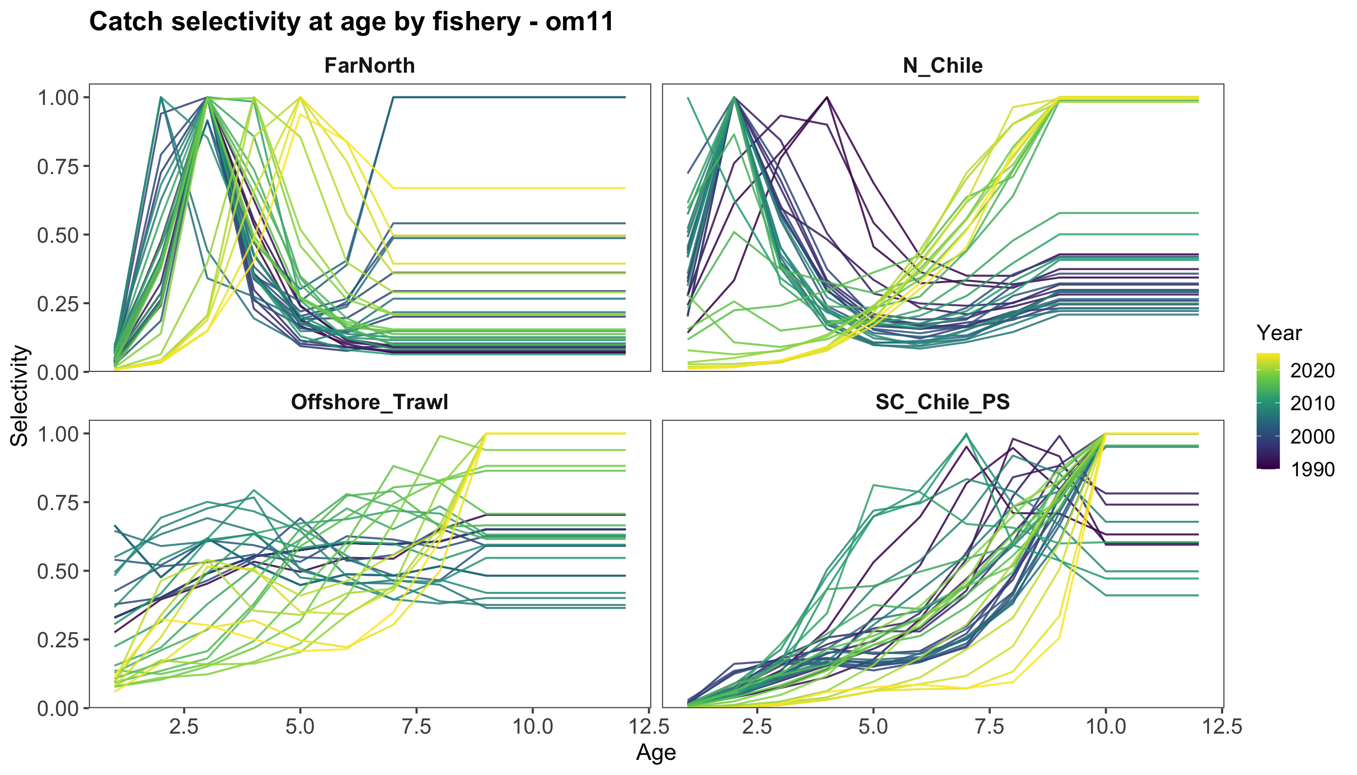
# Selectivity History
The first diagnostic summarizes historical catch selectivity at age by fishery and stock.
This context is important because future projections freeze or average historical selectivity patterns, so changes in recent selectivity can affect projected spawning biomass and catch.
```{r}
#| label: fig-selectivity-history
#| fig-cap: "Historical selectivity-at-age time series used to interpret the projection selectivity assumptions."
#| fig-width: 14
#| fig-height: 8
plot_qmd_selectivity(selex_ts_dt, ref_om=REF_OM)
```
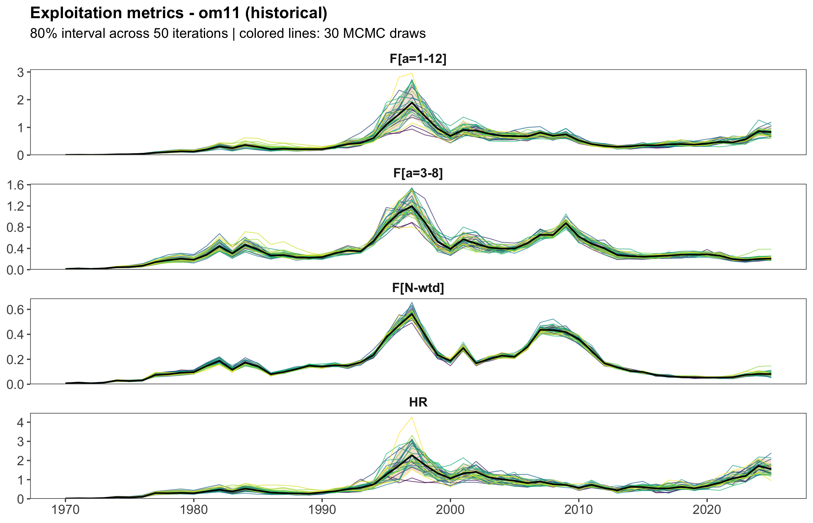
# Historical Exploitation Metrics
The exploitation diagnostic compares alternative fishing mortality or harvest-rate summaries through the historical period.
These metrics provide context for the current fishing mortality level used by the `F2025` scenario.
```{r}
#| label: fig-exploitation-metrics
#| fig-cap: "Historical exploitation metrics for the selected operating model."
#| fig-width: 14
#| fig-height: 9
plot_qmd_exploitation(mets_dt, mets_worms_dt, init_year=INIT_YEAR,
  n_iter=N_ITER, ref_om=REF_OM)
```
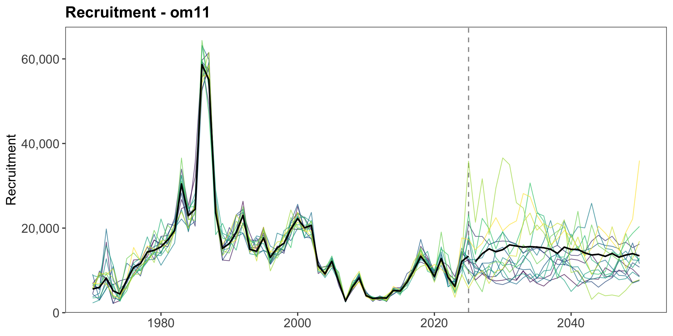
# Recruitment
The recruitment diagnostic shows the historical and future recruitment trajectories used in the projected operating model.
The dashed vertical line marks the final historical year.
```{r}
#| label: fig-recruitment
#| fig-cap: !expr paste("Historical and future recruitment for the selected operating model. The future portion uses the F = 0 projection. Colored lines show", length(unique(rec_worms_plot_dt$iter)), "sampled MCMC draws.")
#| fig-width: 12
#| fig-height: 6
rec_worm_plot_iters <- sort(unique(rec_worms_dt$iter))[seq_len(min(15,
  length(unique(rec_worms_dt$iter))))]
rec_worms_plot_dt <- as.data.table(rec_worms_dt)[iter %in% rec_worm_plot_iters]
plot_qmd_recruitment(rec_dt, rec_worms_plot_dt, init_year=INIT_YEAR,
  final_year=FINAL_YEAR, ref_om=REF_OM)
```
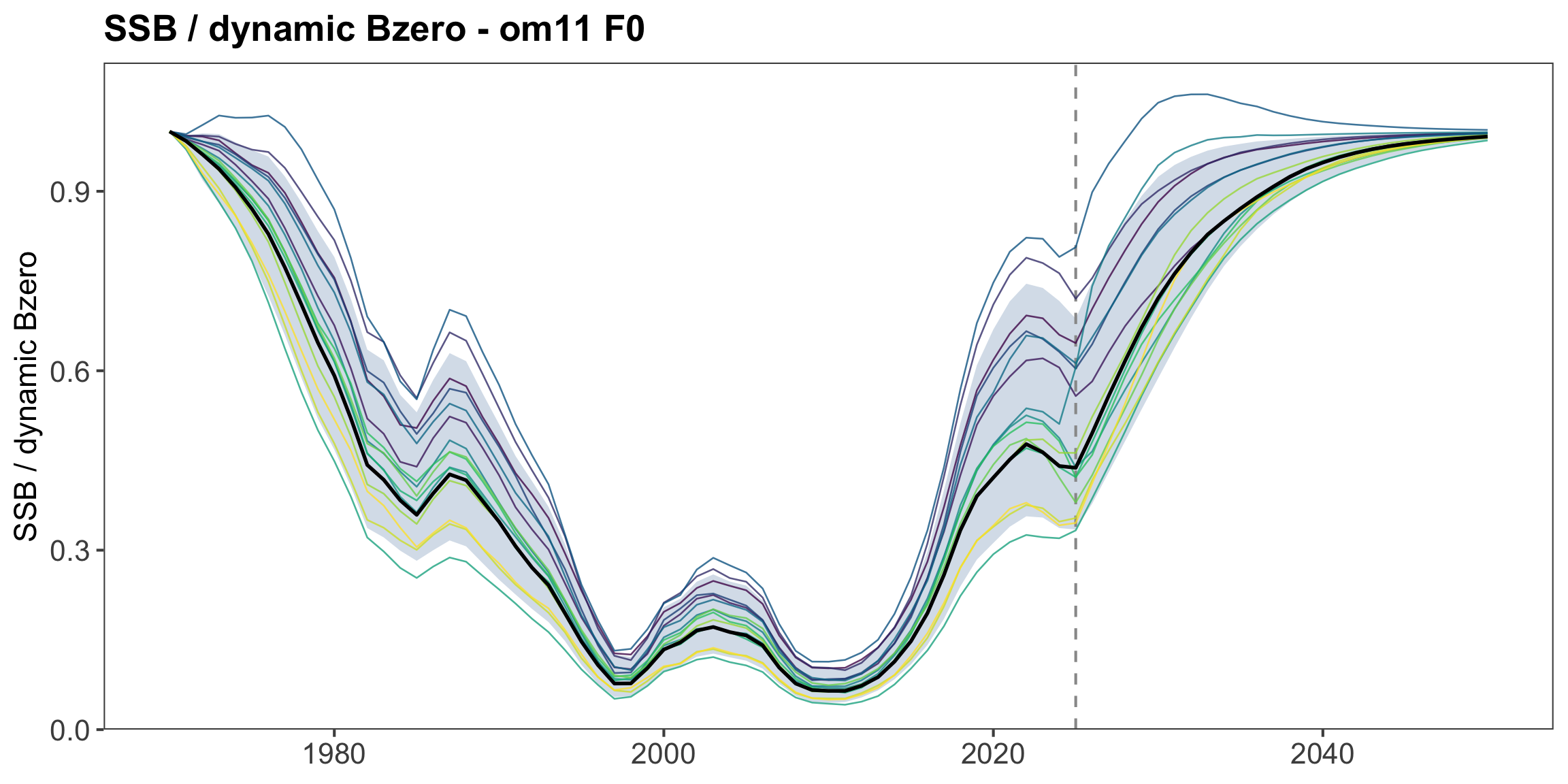
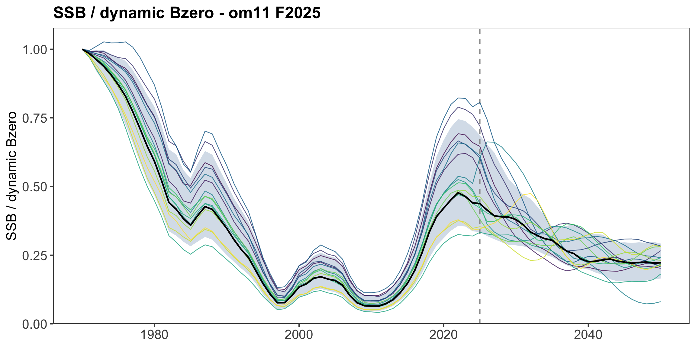
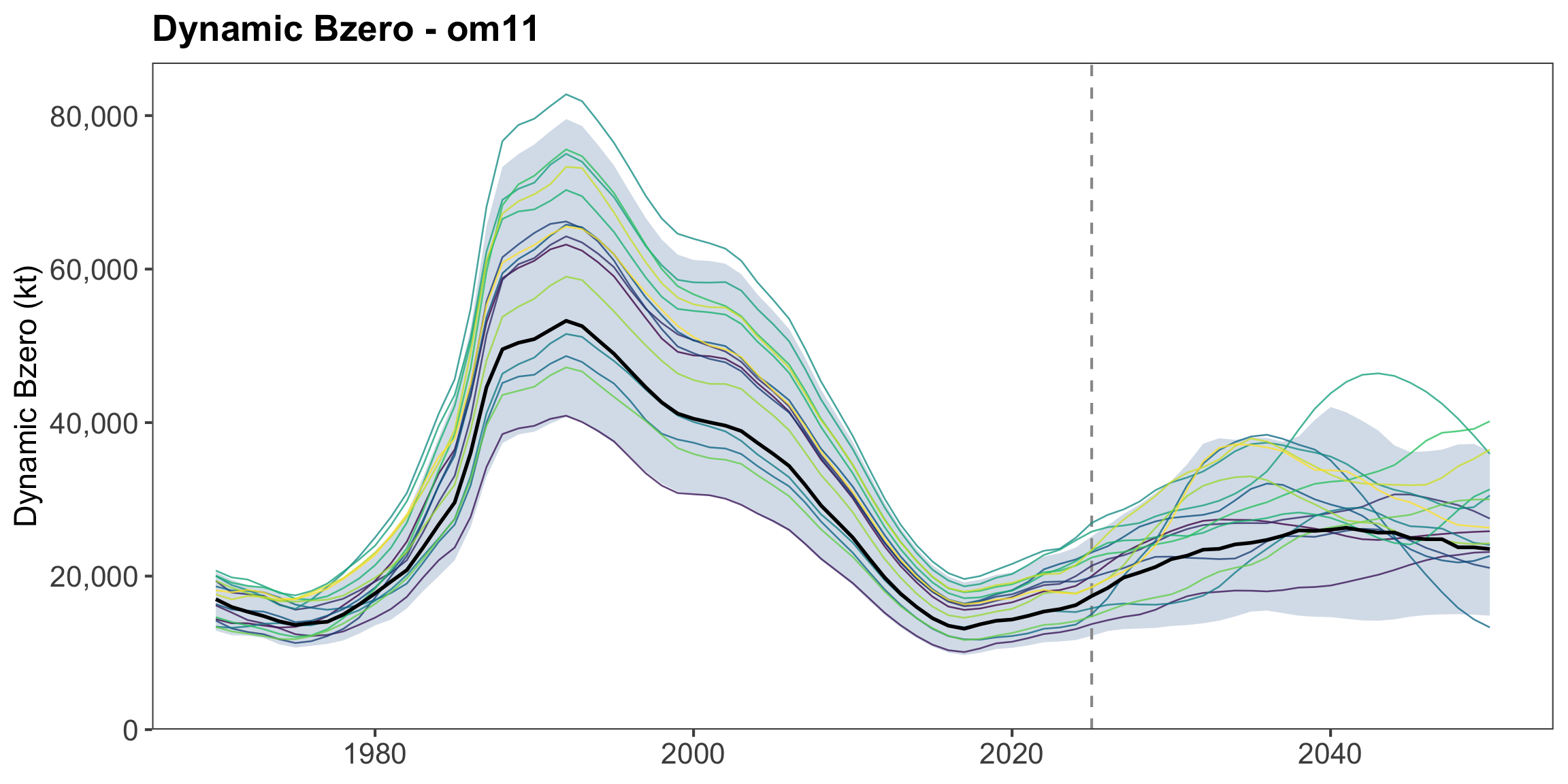
# SSB / Dynamic Bzero
This diagnostic shows SSB relative to the dynamic unfished spawning biomass
trajectory used to scale the terminal stock-status comparison.
The future portion uses the `F0` projection for the selected operating model.
```{r}
#| label: fig-dynamic-bzero
#| fig-cap: !expr paste0("SSB / dynamic Bzero for ", REF_OM, " through ", FINAL_YEAR, ". The future portion uses the F = 0 projection. The ribbon shows the 90% interval across cached MCMC draw trajectories, the black line shows the median, and colored lines show 15 sampled MCMC draws.")
#| fig-width: 12
#| fig-height: 6
plot_qmd_ssb_dynamic_bzero(futs_worms_dt, REF_OM, N_ITER, INIT_YEAR,
  FINAL_YEAR, scenario_filter="F0", worm_n=15)
```
```{r}
#| label: fig-dynamic-bzero-f2025
#| fig-cap: !expr paste0("SSB / dynamic Bzero for ", REF_OM, " through ", FINAL_YEAR, ". The future portion uses the projection with F set equal to the 2025 value. The ribbon shows the 90% interval across cached MCMC draw trajectories, the black line shows the median, and colored lines show 15 sampled MCMC draws.")
#| fig-width: 12
#| fig-height: 6
plot_qmd_ssb_dynamic_bzero(futs_worms_dt, REF_OM, N_ITER, INIT_YEAR,
  FINAL_YEAR, scenario_filter="F2025", worm_n=15)
```
```{r}
#| label: fig-dynamic-bzero-absolute
#| fig-cap: !expr paste0("Dynamic Bzero for ", REF_OM, " through ", FINAL_YEAR, " in kt. The ribbon shows the 90% interval across MCMC draws, the black line shows the median, and colored lines show 15 sampled MCMC draws.")
#| fig-width: 12
#| fig-height: 6
plot_qmd_dynamic_bzero(REF_OM, N_ITER, INIT_YEAR, FINAL_YEAR, worm_n=15)
```
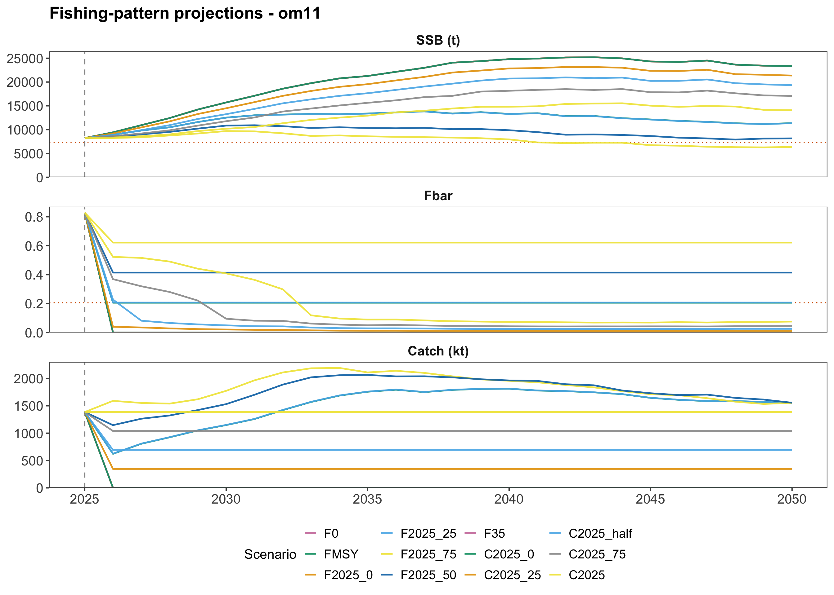
# Future Fishing Pattern Scenarios
The main projection comparison applies the fishing-pattern controls over the projection horizon.
The plot shows median trajectories by scenario for the cached projection summaries, including spawning biomass, fishing mortality, and catch where available.
```{r}
#| label: fig-fixed-scenarios
#| fig-cap: !expr scenario_caption()
#| fig-width: 14
#| fig-height: 10
futs_excluded <- median_fbar_exclusions(
  as.data.table(futs_dt)[year > INIT_YEAR], "scenario")
futs_plot_dt <- drop_group_stock(futs_dt, futs_excluded, "scenario")

plot_qmd_scenarios(futs_plot_dt, INIT_YEAR, sbmsy_ref, fmsy_ref,
  final_year=FINAL_YEAR, ref_om=REF_OM)
```
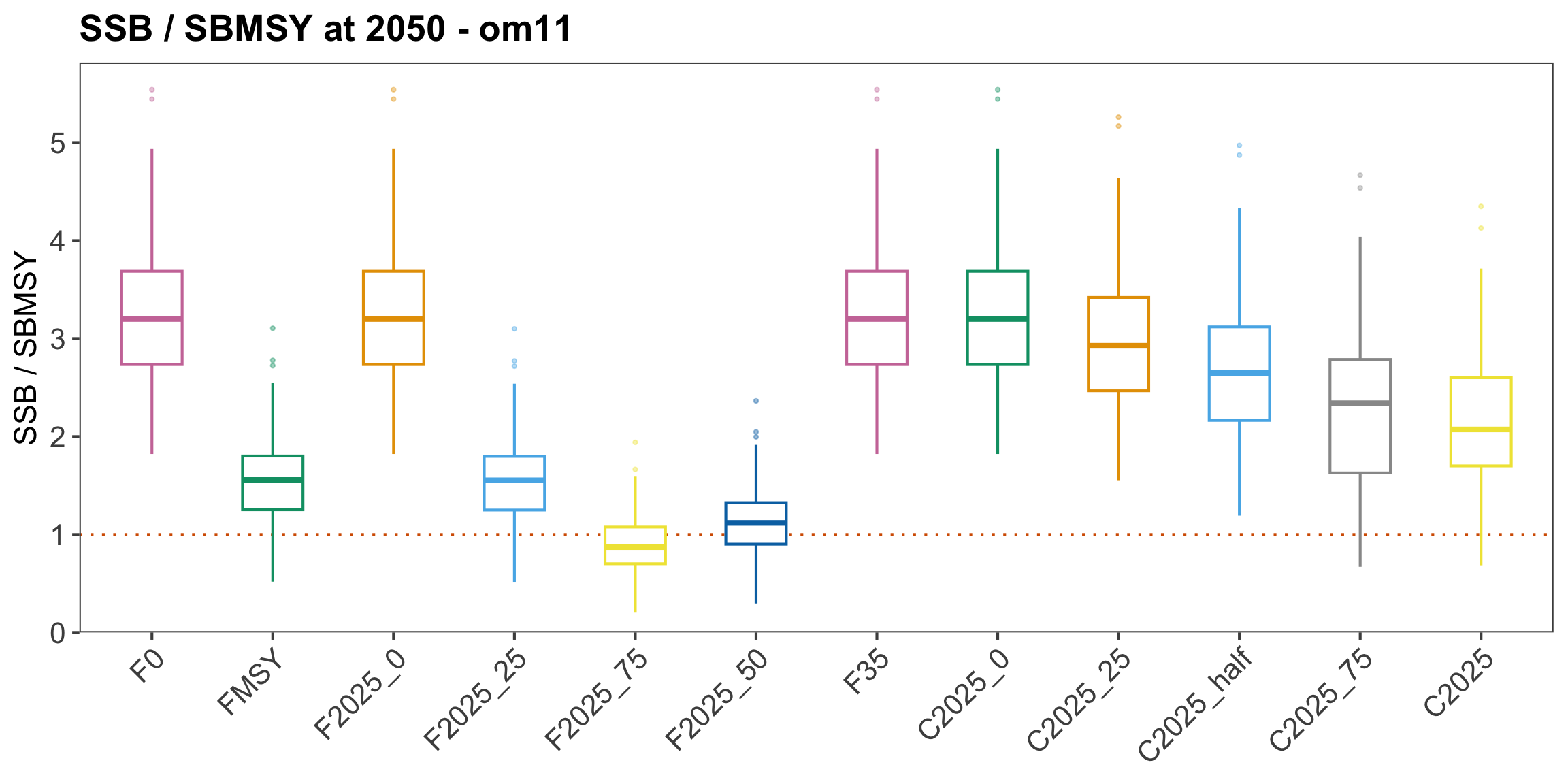
The terminal-status plot shows the distribution of projected spawning biomass relative to SBMSY in the final projection year.
This gives a compact comparison of scenario risk at the end of the projection horizon.
```{r}
#| label: fig-terminal-status
#| fig-cap: !expr paste("Distribution of SSB / SBMSY in", FINAL_YEAR, "under each projection scenario.", N_ITER, "iterations. The dotted line marks SBMSY.", filter_note)
#| fig-width: 12
#| fig-height: 6
status_plot_dt <- drop_fbar_iterations(status_dt, futs_fbar_max_dt, "scenario")
plot_qmd_status(status_plot_dt, FINAL_YEAR, n_iter=N_ITER, ref_om=REF_OM)
```
```{r}
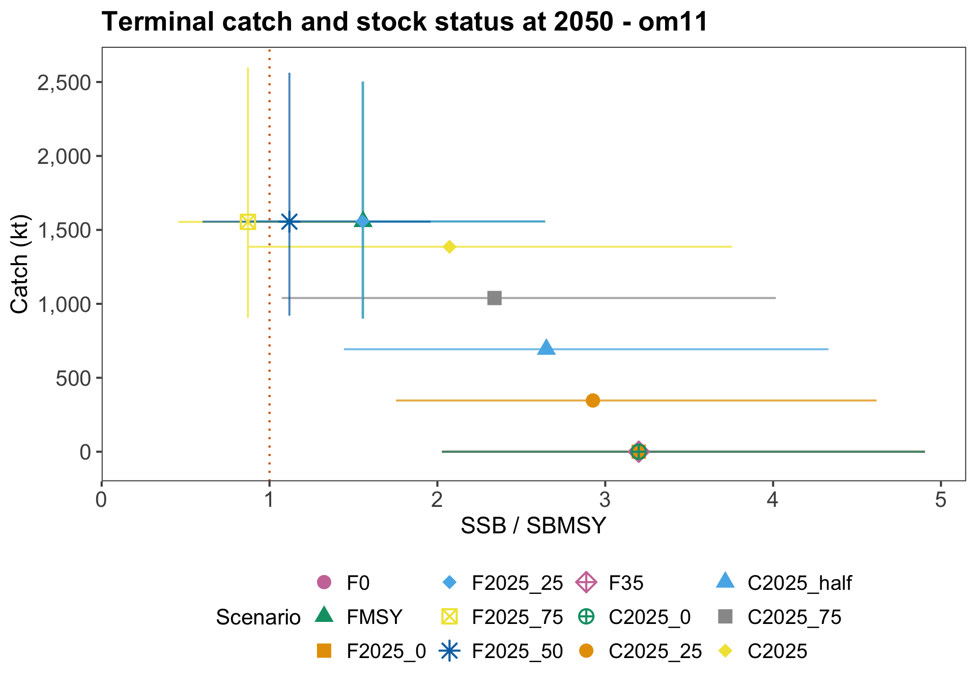
#| label: fig-terminal-tradeoff
#| fig-cap: !expr paste("Median catch and SSB / SBMSY in", FINAL_YEAR, "under each projection scenario. Points show scenario medians; bars show 90% intervals. The dotted line marks SBMSY.", filter_note)
#| fig-width: 10
#| fig-height: 7
plot_qmd_tradeoff(status_plot_dt, FINAL_YEAR, ref_om=REF_OM)
```
```{r}
#| label: fig-terminal-tradeoff-ssb
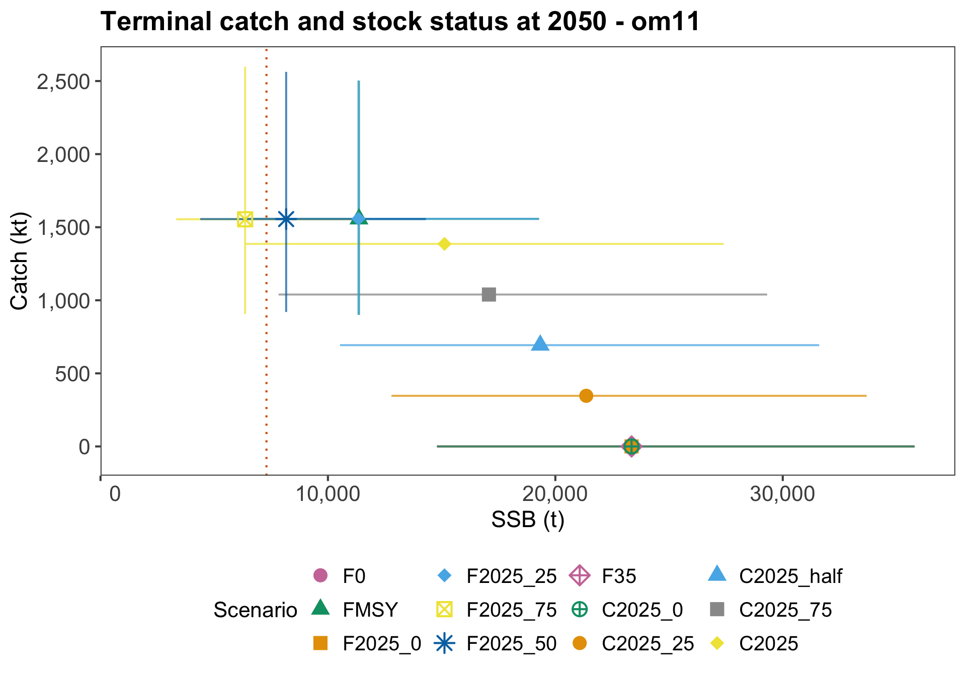
#| fig-cap: !expr paste("Median catch and SSB in", FINAL_YEAR, "under each projection scenario. Points show scenario medians; bars show 90% intervals. The dotted line marks SBMSY.", filter_note)
#| fig-width: 10
#| fig-height: 7
plot_qmd_tradeoff(status_plot_dt, FINAL_YEAR, ref_om=REF_OM,
  x_metric="ssb")
```
```{r}
#| label: fig-terminal-tradeoff-scaled-om11
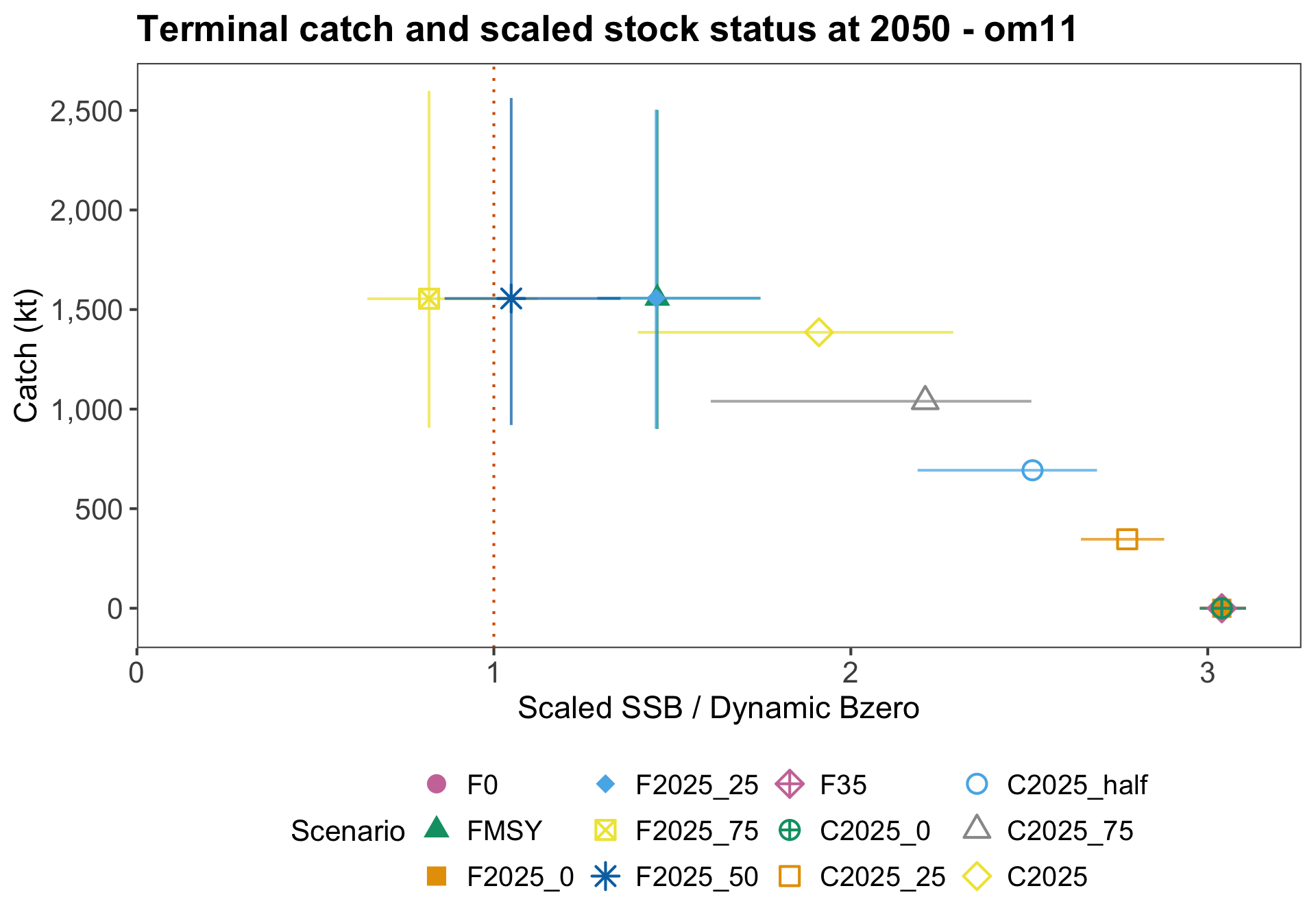
#| fig-cap: !expr paste("Median catch and scaled stock status in", FINAL_YEAR, "under each projection scenario for om11. The x-axis is (SSB / dynamic Bzero) divided by the draw-specific Bmsy / Bzero value. Points show scenario medians; bars show 90% intervals. The dotted vertical line marks the draw-specific Bmsy / Bzero level.", filter_note)
#| fig-width: 10
#| fig-height: 7
scaled_tradeoff_om11_dt <- scaled_tradeoff_data(status_dt, futs_fbar_max_dt,
  REF_OM, N_ITER)
plot_qmd_scaled_tradeoff(scaled_tradeoff_om11_dt, FINAL_YEAR, ref_om=REF_OM)
```
```{r}
#| label: fig-terminal-tradeoff-scaled-om12
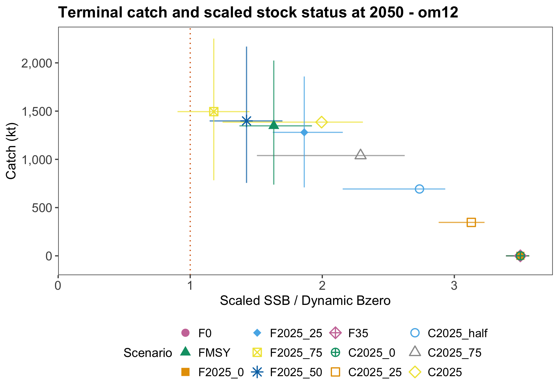
#| fig-cap: !expr paste("Median catch and scaled stock status in", FINAL_YEAR, "under each projection scenario for om12, the steepness = 0.8 operating model. The x-axis is (SSB / dynamic Bzero) divided by the draw-specific Bmsy / Bzero value. Points show scenario medians; bars show 90% intervals. The dotted vertical line marks the draw-specific Bmsy / Bzero level.", filter_note)
#| fig-width: 10
#| fig-height: 7
om12_cache_file <- file.path(jmMSE_path, "report", "projections_om12",
  "cache.rda")
if(!file.exists(om12_cache_file)) {
  stop("OM12 projection cache not found at ", om12_cache_file,
    ". Run explore_projections.R with REF_OM set to 'om12' before rendering.")
}
om12_cache <- new.env(parent=emptyenv())
load(om12_cache_file, envir=om12_cache)
scaled_tradeoff_om12_dt <- scaled_tradeoff_data(om12_cache$status_dt,
  om12_cache$futs_fbar_max_dt, om12_cache$REF_OM, om12_cache$N_ITER)
plot_qmd_scaled_tradeoff(scaled_tradeoff_om12_dt, om12_cache$FINAL_YEAR,
  ref_om=om12_cache$REF_OM)
```
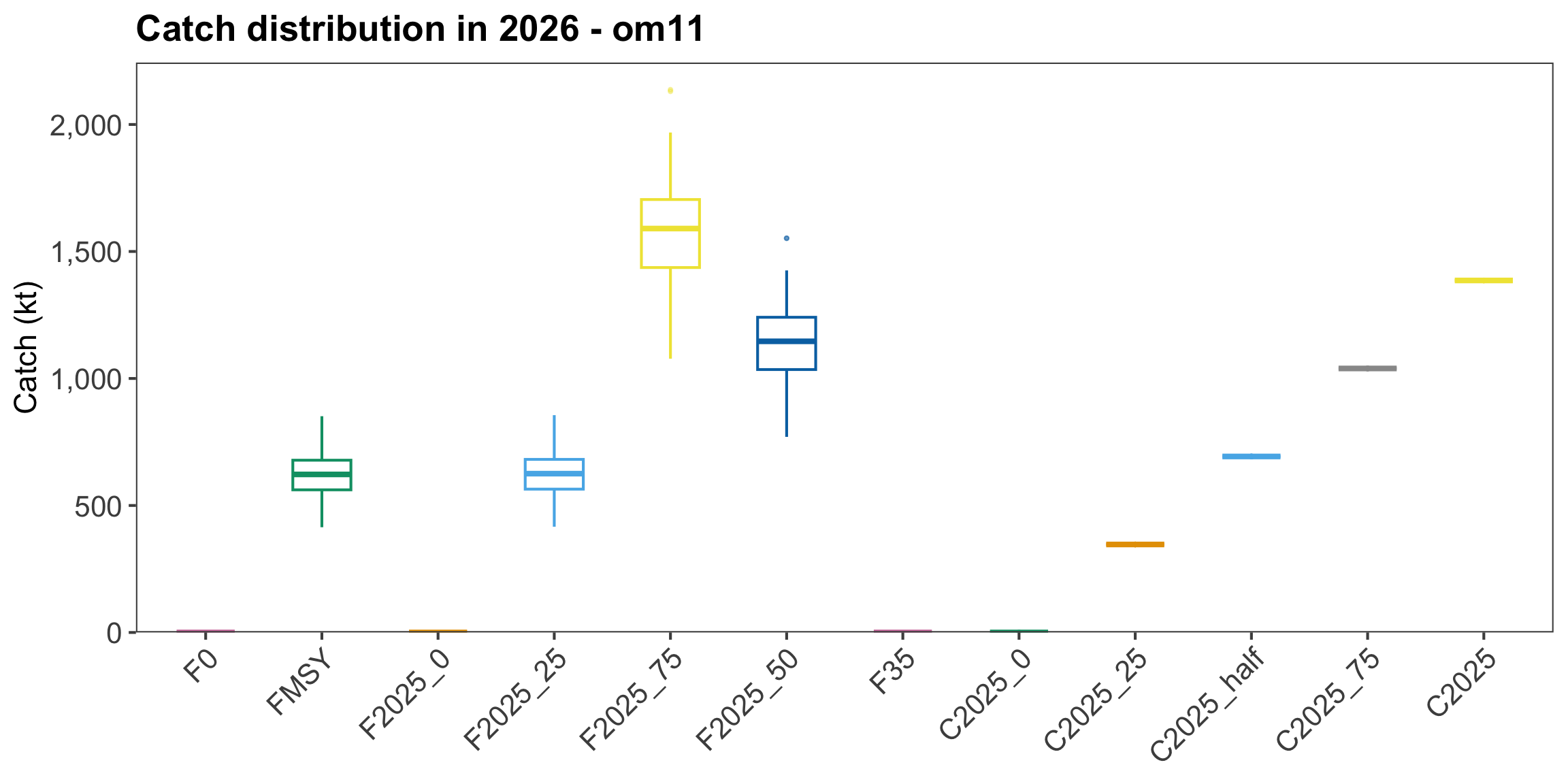
```{r}
#| label: fig-catch-2026
#| fig-cap: !expr paste("Distribution of catch in 2026 under each projection scenario.", N_ITER, "iterations.", filter_note)
#| fig-width: 12
#| fig-height: 6
catch_2026_plot_dt <- drop_fbar_iterations(catch_2026_dt,
  futs_fbar_max_dt, "scenario")
plot_qmd_catch_distribution(catch_2026_plot_dt, 2026,
  n_iter=N_ITER, ref_om=REF_OM)
```
# Selectivity Window Sensitivity
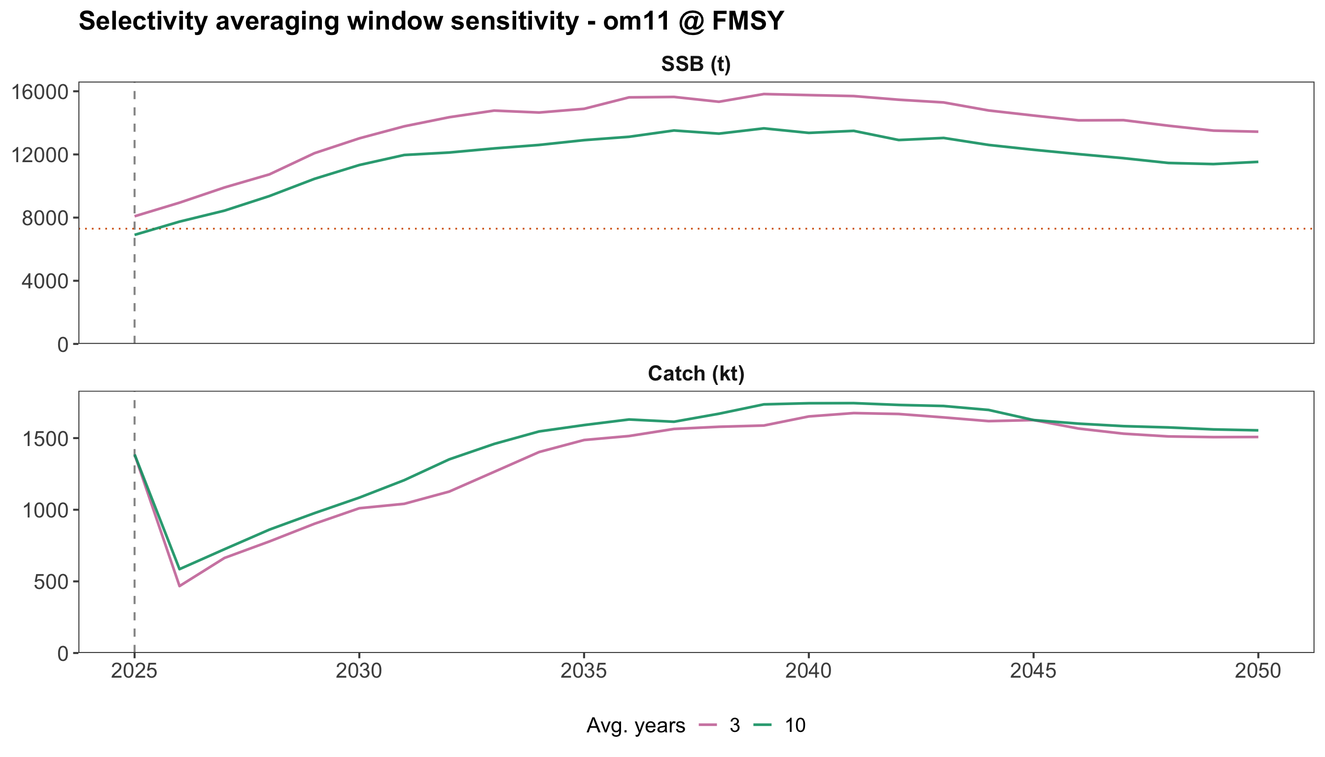
The selectivity-window sensitivity analysis projects at FMSY while replacing future selectivity with averages over alternative terminal-year windows.
For example, a three-year window uses the mean selectivity pattern from the final three historical years.
```{r}
#| label: tbl-selectivity-windows
#| tbl-cap: "Terminal-year selectivity averaging windows."
window_tbl <- data.frame(
  window_years = SELEX_WINDOWS,
  description = paste("Mean selectivity over the final", SELEX_WINDOWS, "historical years")
)

kable(window_tbl, col.names=c("Window (years)", "Projection assumption"))
```
```{r}
#| label: fig-selectivity-window-sensitivity
#| fig-cap: !expr sensitivity_caption("Sensitivity of projections to the terminal-year selectivity averaging window.")
#| fig-width: 14
#| fig-height: 8
selex_excluded <- selex_fbar_max_dt[
  , .(max_median_fbar=median(max_fbar, na.rm=TRUE)),
  by=.(window, stock)][max_median_fbar > FBAR_MAX]
selex_plot_dt <- drop_group_stock(selex_dt, selex_excluded, "window")

plot_qmd_sensitivity(selex_plot_dt, group_col="window", group_lab="Avg. years",
  init_year=INIT_YEAR, sbmsy_ref=sbmsy_ref, fmsy_ref=fmsy_ref,
  ref_om=REF_OM,
  title_prefix="Selectivity averaging window sensitivity")
```
# Selectivity Block Sensitivity
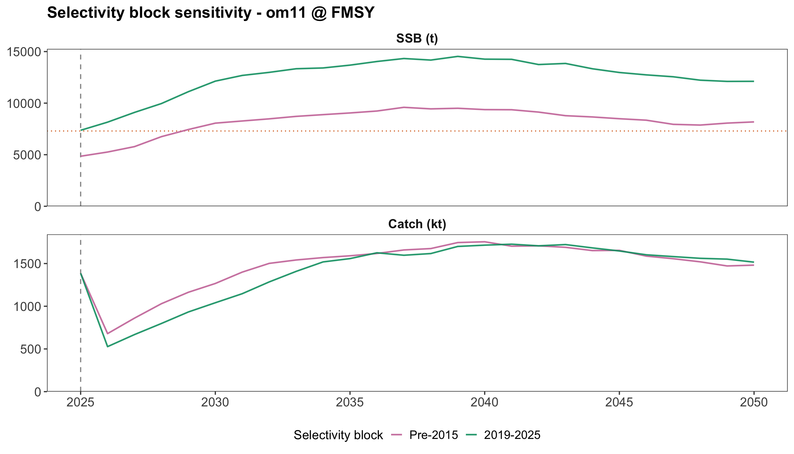
The named-block sensitivity analysis is similar to the rolling-window analysis, but the averaged selectivity pattern comes from specified historical year blocks.
This is useful when historical periods represent different fishery or stock-selectivity regimes.
```{r}
#| label: tbl-selectivity-blocks
#| tbl-cap: "Named historical selectivity blocks used for projection sensitivity."
kable(block_tbl, col.names=c("Block", "Years"))
```
```{r}
#| label: fig-selectivity-block-sensitivity
#| fig-cap: !expr sensitivity_caption("Sensitivity of projections to named historical selectivity blocks.")
#| fig-width: 14
#| fig-height: 8
block_excluded <- block_fbar_max_dt[
  , .(max_median_fbar=median(max_fbar, na.rm=TRUE)),
  by=.(block, stock)][max_median_fbar > FBAR_MAX]
block_plot_dt <- drop_group_stock(block_dt, block_excluded, "block")

plot_qmd_sensitivity(block_plot_dt, group_col="block", group_lab="Selectivity block",
  init_year=INIT_YEAR, sbmsy_ref=sbmsy_ref, fmsy_ref=fmsy_ref,
  ref_om=REF_OM,
  title_prefix="Selectivity block sensitivity")
```
# Outputs
The cached projection workflow writes two main files:
- `report/projections/cache.rda`, containing the settings, summary values, and plot objects used by this report; and
- `report/projections/projections_report.html`, the original HTML report built by `report_run_projections.R`.
This Quarto document provides an editable report source for the same projection results.