| Stage | Date | Identifiers | Material change | Decision status |
|---|---|---|---|---|
| SCW17 Day 4 | 2026-06-18 | run18; run20; run22 | Retained a high-target base case, a minimum-catch case, and a special-shape case from the broader workshop trials | Selected by the workshop for post-workshop robustness testing; not a final CMP selection |
| Post-workshop family refinement | 2026-06 to 2026-07 | MP16; MP25; MP29; MP32 | Added the five-index combination, corrected the power-ramp implementation, adopted the 2019-2023 reference period, and refined minimum and index-limit settings | Analytical development; the workshop run identifiers do not map one-to-one to the later MP identifiers |
| Task-team interpretation | 2026-07-24 | MP29; MP32 | Recorded the stability-responsiveness contrast and remaining work; avoided treating within-family representatives as globally optimal | Draft meeting record; did not select a final CMP |
| Annual-limit comparison | after 2026-07-24 | MP43-MP48 | Added reverse-asymmetric, symmetric, and 30-percent-decrease limits; each variant received its own trigger | Analyst-added comparison awaiting Task Team and Scientific Committee review |
| Common 500-draw refinement | 2026-08 | MP29; MP43; MP45; MP47; MP32; MP44; MP46; MP48 | Retuned all eight controls with the same 500 posterior draws and ran the reference plus nine robustness OMs | Complete analytical comparison; roles are focal, sensitivity, or comparison cases, not a shortlist |
| Named SC14 release candidate | 2026-08-09 | SC14-MSE-2026-RC1 | Aligned CMP registry, results, figures, scorecards, downloads, Slick contents, papers, run list, and file fingerprints | All automatic agreement checks passed; SC14 decision remains outstanding |
Jack mackerel management strategy evaluation for SC14
Operating models, candidate management procedures, robustness tests, and matters for Scientific Committee consideration
Jack Mackerel Management Strategy Evaluation: Synthesis for SC14
Status and purpose. This is a working pre-submission revision based on the scientific outputs frozen in SC14-MSE-2026-RC1. The revised documents and new review-evidence tables are not part of that fingerprinted release; they require a new release candidate after review. The report synthesizes the June 2026 SCW17 MSE workshop and subsequent model and management-procedure development.
Executive summary
The jack mackerel MSE has progressed from a broad workshop design into a narrower comparison of candidate management procedures (CMPs) tested against a reference operating model (OM) and a structured set of robustness OMs. SCW17 established the principal design choices: simple and interpretable empirical rules, simulation of correlated index errors, dynamic reference points, explicit robustness testing, a broad performance-measure set, and development of an exceptional-circumstances protocol. Post-workshop work corrected and extended the implementation, tuned the leading rule families, and examined their performance under one-stock and two-stock hypotheses, recruitment stress, movement, selectivity, and alternative annual TAC-change limits.
A novel feature of this MSE is its treatment of the five abundance indicators as related observations rather than independent sources of information. The OMs simulate their observation errors jointly using historical estimates of each series’ uncertainty, temporal autocorrelation, and cross-correlation. This allows the evaluation to represent shared movements among indicators, including correlation that may arise when the population shifts spatially. The estimated correlation structure used for the reference OM is illustrated in Figure 1.
Among the dozens of MPs evaluated at the SCW17 workshop, the analysts concluded that the hockey-stick and power-ramp designs represented by these two CMPs, together with reasonable variants of those designs, were suitable to carry forward as proposals for consideration at SC14. This analytical conclusion identifies a focused set for Scientific Committee consideration; it is not a formal recommendation or adoption decision.
The main Jack Mackerel MSE resource page describes the naming conventions and how the MSE components fit together, and provides the CMP and OM registries and translation tables linking the labels used across analyses and reports.
Two CMPs are the focal cases for the current comparison:
- HS-20 (MP43) uses a hockey-stick harvest control rule (HCR), a 2,000-kt catch target, a 270-kt minimum, and annual limits of a 20% decrease and 15% increase.
- PR-20 (MP44) uses a power-ramp HCR, a 1,500-kt catch target, the same minimum, and the same annual limits, with a more responsive reduction in advice as the indicator declines, and the ability to increase catches above the target level.
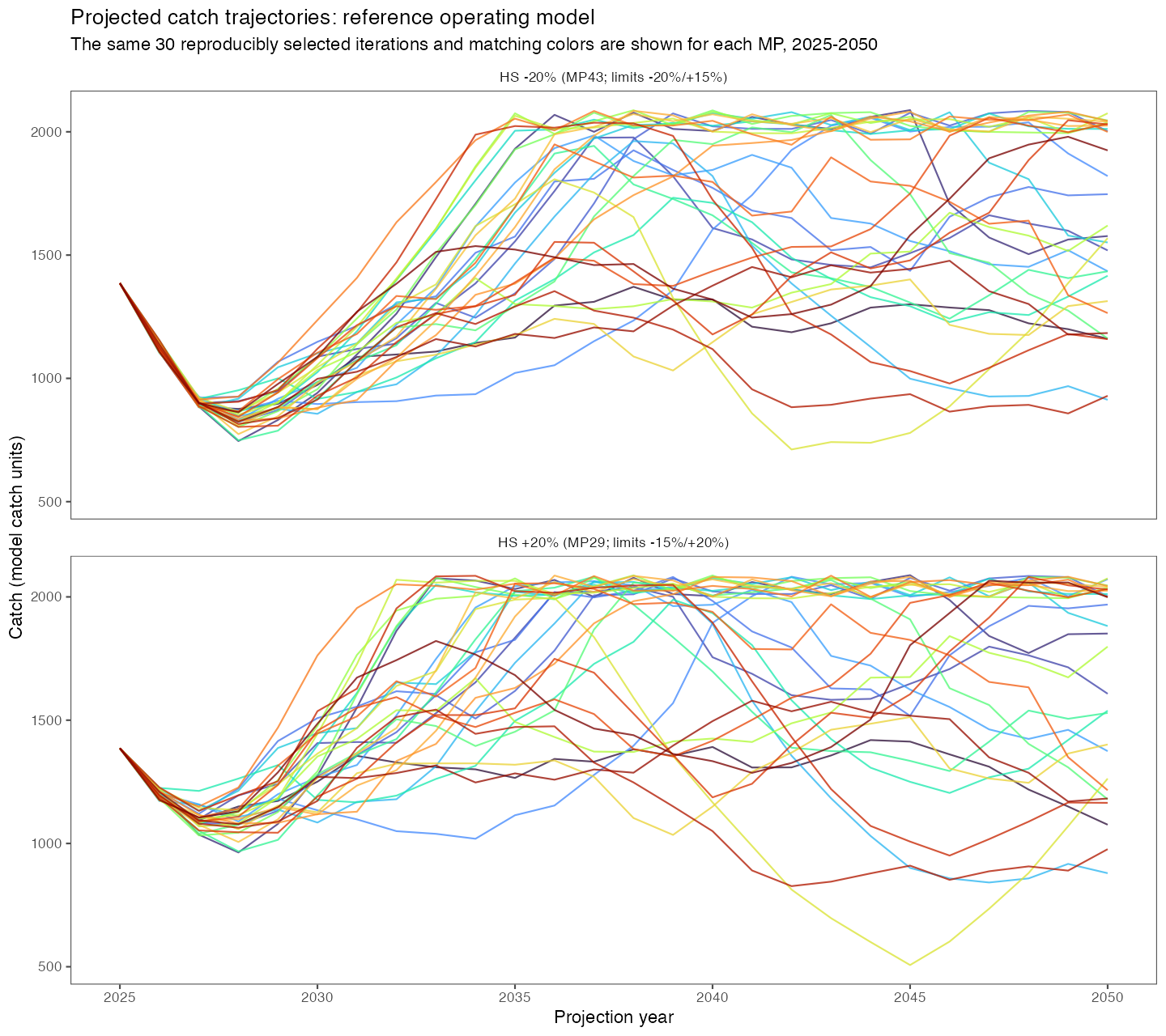
Both use the combined indicator assembled from five standardized abundance indices. The earlier HS+20 (MP29) and PR+20 (MP32) specifications are retained as sensitivity cases. They arose from an initial request informed by early feedback from Chile’s internal MSE research project; their 20% maximum annual TAC increase was not selected from the later Commission poll. That poll helped inform the broader set of annual TAC-change variants examined here. The remaining HSsym, HS-30, PRsym, and PR-30 procedures are additional comparison cases. The paired catch trajectories for focal HS-20 and sensitivity HS+20 illustrate one annual-limit contrast in Figure 4.
The scorecard is retained as a preliminary sensitivity tool rather than an executive ranking. Its ordering changes with the candidate set, metrics, directions, scaling, and weights; it does not determine biological acceptability, focal status, or a shortlist. Raw outcomes, uncertainty, and performance under individual OMs remain the primary evidence.
All eight CMPs were refined against the same 500 posterior draws to target an approximately 60% mean probability of dynamic Kobe-green status during 2041–2050. Their realized probabilities range from 59.2% to 61.0%, so the comparison is now like-for-like with respect to the tuning objective. The archived 100-draw results remain useful provenance but are superseded by the 500-draw reference and robustness results used throughout this report. The earlier comparisons reviewed on 24 July identified a broad contrast between the stability of the hockey-stick family and the stronger response of the power-ramp family as indicators declined. The completed results refine that comparison across all eight CMPs; differences depend on the OM and performance measure and do not establish a preferred or “optimal” CMP.
The most consequential robustness finding came from the two-stock hypotheses. Without movement, the southern component passed the agreed benchmark while the northern component required an exploratory change of ~3% in simulated catch distribution from north to south to reach the same benchmark. This is a sensitivity result, not an allocation recommendation. With movement, no tested fixed catch distribution achieved the long-term benchmark for both components. Equal weighting of indices could also mask a declining southern component when northern indices increased. Separate annual tracking of northern and southern indices is therefore an important candidate element of exceptional-circumstances monitoring.
The Scientific Committee is asked to consider the adequacy of HS-20 (MP43) and PR-20 (MP44) as the focal cases; the role of HS+20 (MP29) and PR+20 (MP32) as sensitivity cases; the other annual TAC-change variants to retain; the role of all five indices, including the only fishery-independent series; the interpretation of two-stock robustness; the completed 500-draw reference and robustness evaluation; and the work needed to validate and complete banking-and-borrowing and exceptional-circumstances evaluation.
1 Purpose, scope, and decision status
The MSE is intended to compare complete management procedures in a closed-loop simulation before one is considered for implementation. Each CMP converts agreed observations into annual catch advice; each OM represents a plausible description of stock and fishery dynamics against which the CMP is tested. Performance measures describe biological outcomes, yield, stability, and fishery feasibility over specified periods.
This report melds the technical foundation assembled in the benchmark-preparation and MSE-planning materials, the design record from the SCW17 MSE Workshop report, and the post-workshop analysis summarized in the final 24 July task-team meeting report and the presentation from Wageningen Marine Research consultants (WUR). The preparation site preceded SCW17 and provided the detailed model specifications, diagnostics, working papers, and technical discussions needed to update the operating models used at SCW17 and in subsequent MSE work. Their different roles are summarized in Table 1.
| Source | Role in this synthesis |
|---|---|
| Benchmark preparation and MSE planning | Pre-SCW17 benchmark papers, OM specifications, diagnostics, index analyses, and preparatory meeting records that supported updates to the OMs used at SCW17 and beyond. |
| SCW16 benchmark report | Formal record of the May 2026 benchmark review, including assessment inputs, abundance indices, biological assumptions, model alternatives, decisions, and uncertainties to carry into OM conditioning. |
| SCW17/Paper-01: Model developments | Post-SCW16, pre-SCW17 bridge from the benchmark model sequence to the 0.15 and 0.16 configurations considered for MSE conditioning, with model comparisons and diagnostics. |
| SCW17 workshop report, 15–19 June 2026 | Agreed MSE design, OM and CMP principles, reference-point approach, performance framework, and planned robustness work. |
Post-workshop jmMSE analysis |
Implemented CMP definitions, tuning runs, reference and robustness simulation outputs, and reproducibility records. |
| Task-team meeting, 24 July 2026 | Interpretation of results, wording cautions, issues for SC14, and agreed follow-up. |
| July WUR presentation | Detailed tuning sequence, OM contrasts, and graphical robustness diagnostics available at the time of review. |
| Draft weighted scorecard, 23 July 2026 | Example of an editable multi-criteria comparison method; not an exhaustive candidate list, metric list, or decision. |
The Scientific Committee provides scientific advice and the Commission weighs management trade-offs and makes management decisions. A shortlist in an MSE analysis is not an adoption decision.
2 Development from SCW17 to the current analysis
SCW17 continued work begun at the 2025 SCW15 MSE workshop (SPRFMO Jack Mackerel Working Group 2025) and the 2026 benchmark. The benchmark-preparation and MSE-planning site preserves the detailed model specifications, diagnostics, index working papers, and preparatory meeting discussions that preceded SCW17. That record provided the technical basis for updating the operating models taken into the workshop and used in subsequent MSE analyses.
SCW17 aimed to prepare an OM set, trial CMPs, performance statistics, robustness scenarios, and documentation for SC14. The workshop favored simple empirical rules because they are transparent, reproducible, and can be locked before use. Trial CMPs were used to learn about rule behavior and were not final recommendations.
Post-workshop work made the following material advances:
- Index projection errors were extended to include iteration-specific variability, autocorrelation, and cross-correlation among index deviations.
- Dynamic biological reference points and additional measures, including vulnerable-biomass and exploitation measures, were incorporated.
- A straight-slope comparison rule was added.
- The power-ramp implementation was corrected to remove discontinuities around its limit. The correction was required for consistent implementation but did not overturn the broad workshop conclusions.
- A projected effort constraint was added to avoid implausible catches that would require extreme effort increases from current levels.
- CMP tuning was performed as a nested screen of HCR family, catch target, minimum catch, index limit, index set, simulation replication, and robustness performance.
- Alternative annual TAC-change limits were retuned instead of being compared using triggers tuned under a different constraint.
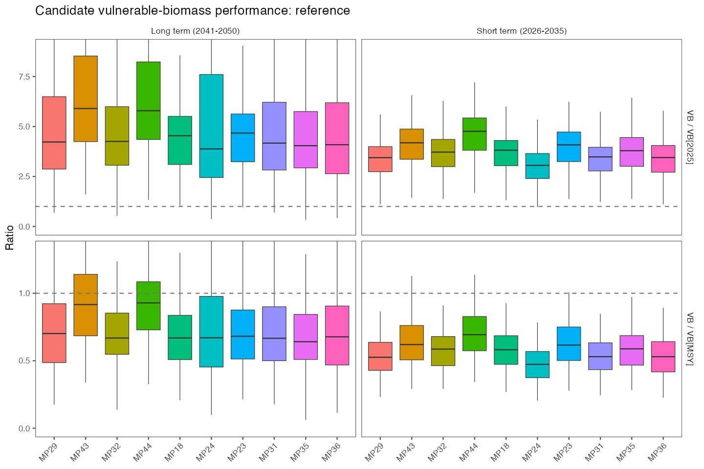
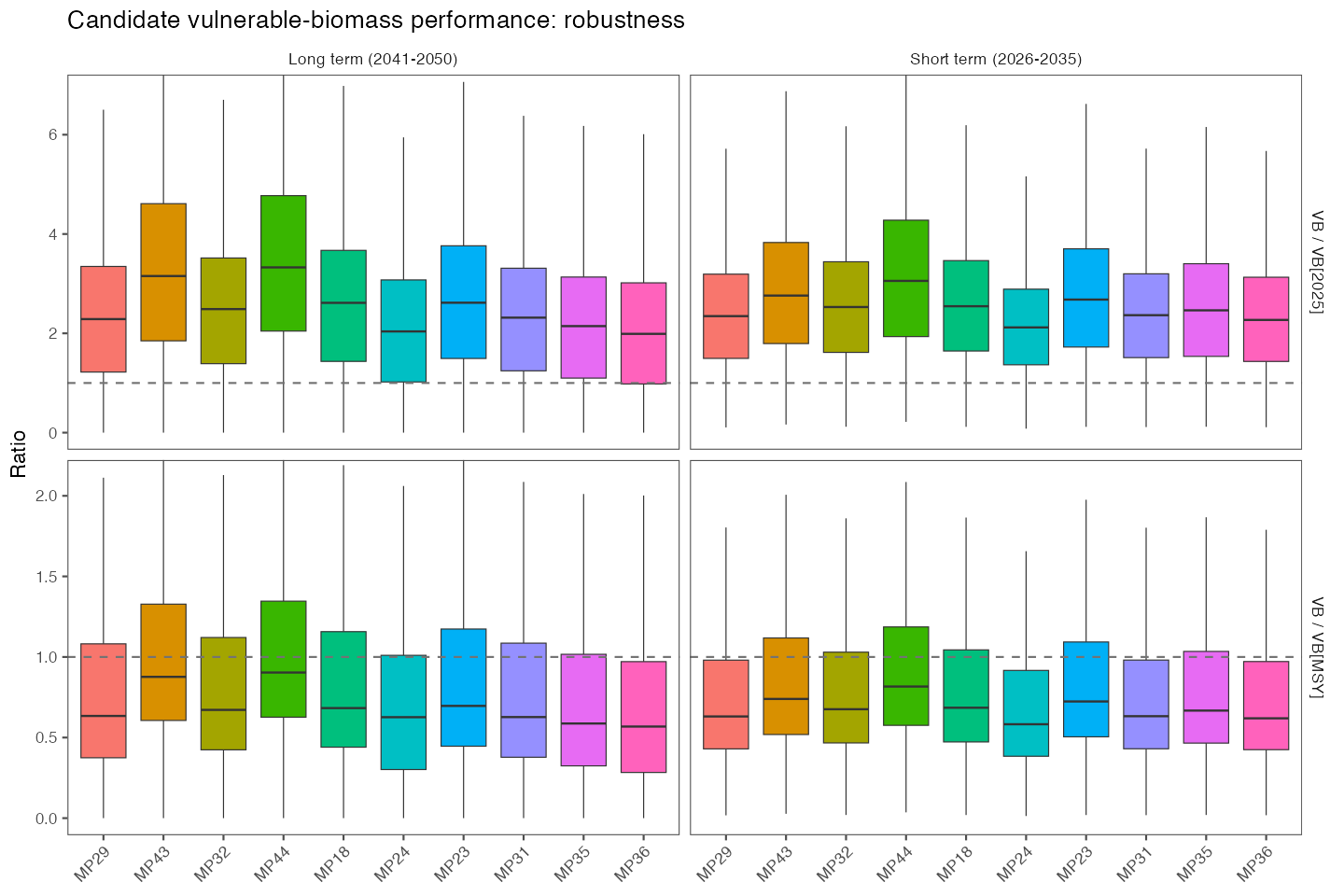
The development of vulnerable-biomass performance indicators responded to a request from SCW17 for a measure that could complement spawning biomass and be more relatable to fishers. In this context, vulnerable biomass represents the fish available to the fishing fleet under the modeled selectivity. It was therefore developed as a fishery-facing performance measure, while spawning biomass remains the principal measure of reproductive stock condition.
The July WUR presentation used the word “optimal” for some within-family runs. The 24 July meeting clarified the interpretation: those runs were useful within-family representatives, but the analysis does not establish an optimal procedure across management objectives.
The sequence from the workshop trials to the current comparison is recorded in candidate-development-history.csv. The workshop run18/run20/run22 subset is an antecedent development set, not a one-to-one renaming of MP29/MP32 or MP43–MP48. The annual-limit variants were added after the 24 July meeting and remain analyst-developed comparison cases awaiting Task Team and Scientific Committee review.
3 Operating models and simulation methods
3.1 Reference and robustness set
The operating-model set did not begin at SCW17. The SCW16 benchmark workshop report records the 18–22 May 2026 review of assessment inputs, abundance indices, biological assumptions, assessment-model alternatives, and priorities for OM conditioning (SPRFMO Jack Mackerel Working Group 2026a). It is the benchmark decision record that defined the assessment foundation and identified which uncertainties should be fixed, retained as OM axes, or examined diagnostically.
Following SCW16 and before the SCW17 workshop, the working group prepared SCW17/Paper-01: Model developments (SPRFMO Jack Mackerel Working Group 2026c). That paper explicitly bridged the SCW16 baseline (0.00) and proposed final benchmark configuration (0.14) to the post-benchmark 0.15 and 0.16 developments. It documented the revised treatment of the Peruvian artisanal and industrial CPUE series, the change to the two-stock productivity-regime specification in 0.16, comparisons with the benchmark anchor models, and diagnostics for the configurations presented for MSE conditioning. SCW17 subsequently used h1_0.16 as the primary basis for CMP testing, retained the matching two-stock configuration for structural robustness, and retained the SC13-era 0.00/1.14 configuration as an assessment/configuration robustness case. Thus, the current OM set should be read as the product of the SCW16 benchmark followed by a documented post-benchmark model-development step, rather than as a set first defined at SCW17.
The current grid centers on the one-stock benchmark model h1_0.16 with steepness 0.65. Robustness OMs test major structural and parametric uncertainties rather than assigning probability to one forecast (Table 3).
| OM label | Main contrast | Analytical role | Proposed decision treatment |
|---|---|---|---|
| om11 | One stock, model 0.16, steepness 0.65 | Reference OM for current tuning | Primary comparison; not assigned a numerical plausibility weight |
| om11_1 | Alternative selectivity | Younger/smaller fish exposed to greater fishing pressure | Structural sensitivity that may affect reference-point interpretation |
| om11_2 | One-year recruitment crash | Acute recruitment stress | Stress test; concern should be reported rather than silently pooled |
| om11_3 | Seven-year cyclic recruitment reduction | Prolonged recruitment stress | Stress test; concern should be reported rather than silently pooled |
| om12 | One stock, steepness 0.8 | Productivity robustness | Parameter sensitivity |
| om13 | One stock, SC13-era/model 1.14 configuration | Assessment/configuration robustness | Legacy-configuration sensitivity |
| om21 | Two stocks, no movement | Stock-structure and catch-distribution robustness | Structural sensitivity requiring component-level results |
| om21_1 | Two stocks with movement | Spatial redistribution and indicator-conflict robustness | Difficult structural case requiring an explicit SC14 judgment |
| om22 | Two stocks, steepness 0.8 | Two-stock productivity robustness | Structural and parameter sensitivity requiring component-level results |
| om23 | Two stocks, model 1.14 configuration | Two-stock assessment/configuration robustness | Difficult legacy-configuration case requiring an explicit SC14 judgment |
The OM set (reference and robustness) is not a declaration that all states are equally plausible. No numerical plausibility weights have been agreed. The proposed treatments above keep the reference comparison, structural sensitivities, and deliberate stress tests distinct while bringing difficult results forward. SC14 should decide whether any case is exclusionary, a source of concern, or informative but non-decisive; any later OM weighting must be explicit and documented.
3.2 Recruitment, observation, and implementation uncertainty
Recruitment variability strongly influences stock trajectories and dynamic reference points. The core simulations therefore retain recruitment uncertainty, while discrete crash and cyclical-reduction cases act as stress tests. SCW17 treated ENSO and climate effects as robustness questions at this stage rather than embedding a single climate forecast in the core OM.
3.3 Dynamic reference points
Environmental recruitment variability can make static reference points misleading. In paragraph 58 of the SCW17 workshop report, the Working Group strongly recommended calculating the ratio \(B_{\mathrm{MSY}}/B_0\) within each MCMC draw, multiplying it by the corresponding dynamic \(B_0\), and evaluating spawning biomass relative to that dynamic \(B_{\mathrm{MSY}}\). The current tuning objective uses a dynamic Kobe-green measure that combines biomass and fishing-pressure status.
Reference-point choices remain consequential. In particular, alternative selectivity can change \(F_{\mathrm{MSY}}\) and therefore \(F/F_{\mathrm{MSY}}\) even when biomass and catch trajectories are similar. Interpretation should separate changes caused by reference-point definitions from changes in underlying CMP behavior.
3.4 Generating OM data indices
Each CMP receives simulated abundance indices rather than true stock status. Projected index deviations include autocorrelation and cross-correlation so that the observation model represents the estimated historical behavior of multiple surveys and CPUE series. The final values and data coverage used by the reference OM are reported below.
The combined indicator does not assume that five series provide five independent confirmations of stock change. In each OM iteration, projected index errors are generated jointly from the historical index deviations: series-specific log-scale standard deviations describe uncertainty, lag-1 parameters preserve temporal autocorrelation, and an iteration-specific correlation matrix preserves cross-correlation among indices. These relationships matter because common environmental effects, fleet behavior, and spatial redistribution of the population can cause several indices to rise or fall together.
For index \(i\) in year \(t\), the log deviation follows \(x_{i,t}=\rho_i x_{i,t-1}+\epsilon_{i,t}\) and the multiplicative observation deviation is \(\exp(x_{i,t})\). The innovation covariance is constructed from the iteration-specific marginal log-scale standard deviations, lag-1 coefficients, and historical cross-correlation matrix. The implementation adjusts the innovation correlation for the AR(1) coefficients and applies a nearest-positive-definite correction before Cholesky simulation when needed. Parameters are estimated separately within each posterior iteration from the available historical index deviations through 2025; Table 4 shows their means across iterations.
| Index | First year | Last year | Years with data | Mean log SD | Mean lag-1 rho |
|---|---|---|---|---|---|
| Chile_AcousN | 1984 | 2025 | 25 | 0.897 | 0.094 |
| Chile_CPUE | 1998 | 2025 | 28 | 0.171 | 0.283 |
| Peru_Artis | 2002 | 2025 | 24 | 0.302 | 0.581 |
| Peru_Ind | 2002 | 2025 | 20 | 0.348 | 0.628 |
| Offshore_CPUE | 2008 | 2024 | 17 | 0.239 | -0.037 |
The five series overlap completely only during 2008–2009, 2011–2014, and 2018–2021. The northern Chile acoustic series has earlier and intermittent coverage, including no 2022 value; the Peruvian industrial series has four historical gaps; and offshore CPUE ends in 2024. These gaps are retained in the estimation data rather than silently filled. The full mean correlation matrix is downloadable as index-error-correlations.csv, and the complete gap list, coverage, and parameter values are in index-error-parameters.csv.
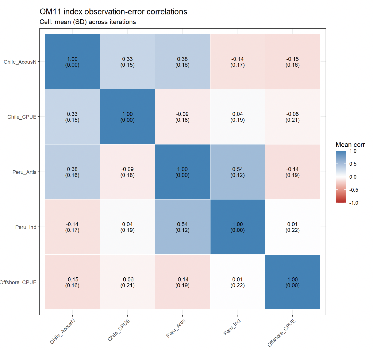
As shown in Figure 1, the estimated relationships are neither uniformly positive nor interchangeable. For example, the Peru artisanal and industrial indices have the strongest positive mean cross-correlation (0.54), whereas several relationships involving the offshore CPUE series are weakly negative. The standard deviations in parentheses show that the observation-error correlation matrix also varies among OM iterations.
The resulting closed-loop test therefore exposes the CMP to realistic combinations of agreement, redundancy, and divergence among indicators. The novelty lies in evaluating the simple, transparent equal-weight composite under this estimated multivariate observation process; equal weighting itself is not covariance weighting and does not mathematically remove correlation. This approach is consistent with the MSE best-practice principle that management procedures should be tested using simulated management data that represent observation uncertainty rather than receiving true stock status (Punt et al. 2016).
This model covers stochastic marginal error, persistence, cross-series correlation, and posterior variation in those estimates. It does not by itself represent gradual catchability drift, abrupt re-standardization, revised historical data, systematic regional imbalance, or reliability-based index weighting. Tests of those mechanisms, missing-survey rules, and region-balanced or reliability-weighted indicators remain continuing work.
4 Candidate management procedures
4.1 Common indicator and annual calculation
The central CMPs use five observed series: northern Chile acoustic biomass, Chilean CPUE, Peruvian artisanal and industrial indices, and offshore CPUE. Each series is expressed relative to its 2019–2023 mean. The standardized values are combined with equal weights within each year, after the OMs have generated the indices using estimated uncertainty, temporal autocorrelation, and cross-correlation among series. The CMP then uses a three-year recent average of the combined indicator.
Most data are assumed to arrive with a one-year lag, while offshore CPUE has a two-year lag. Under the tested timing, a calculation during 2026 for 2027 advice would use 2025 values for the acoustic, Chilean CPUE, and Peruvian indices, and the 2024 offshore CPUE value. Same-year 2026 observations do not enter that tested 2027 calculation unless the timing rule is explicitly changed and re-evaluated, and observations were known to be available in time.
4.2 Naming convention and candidate variants
The working labels encode the HCR family and the most distinguishing annual TAC-change constraint. HS means hockey-stick and PR means power ramp. +20 identifies the base 20% maximum increase, -20 identifies the reverse asymmetry with a 20% maximum decrease, sym identifies symmetric 15% limits, and -30 identifies a 30% maximum decrease. These labels should be used in figures and interpretive prose. The legacy MP identifiers remain in the table only to preserve the link to code, saved outputs, and earlier documents. The complete mapping is given in Table 5.
4.3 Focal cases and annual-limit sensitivities
All eight CMPs use the same five-index mean, 2019–2023 reference period, three-year averaging window, 270-kt minimum catch, 0.1 index limit, and 1,385-kt initial simulated catch. Each variant was refined under the reference OM using the same 500 posterior draws after setting its annual constraint.
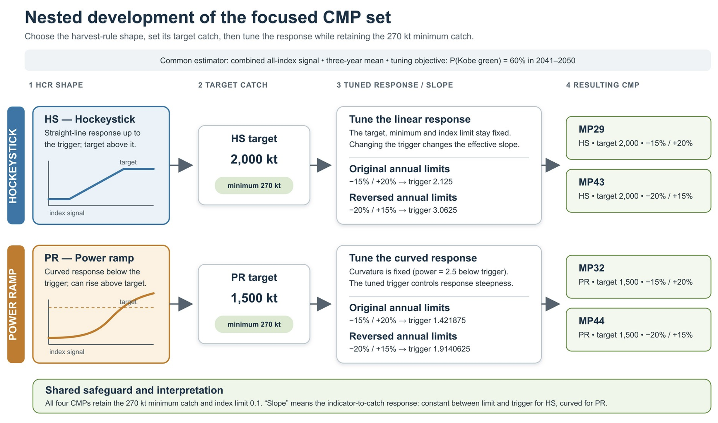
The nested development framework in Figure 2 shows how the focused comparison was constructed: first select the HCR shape, then its target catch, and finally tune the trigger controlling the indicator-to-catch response, while retaining the common minimum catch and index limit. The figure records the earlier 100-draw trigger controls used during development; the subsequent common 500-draw refinement used for current results is reported in Table 5.
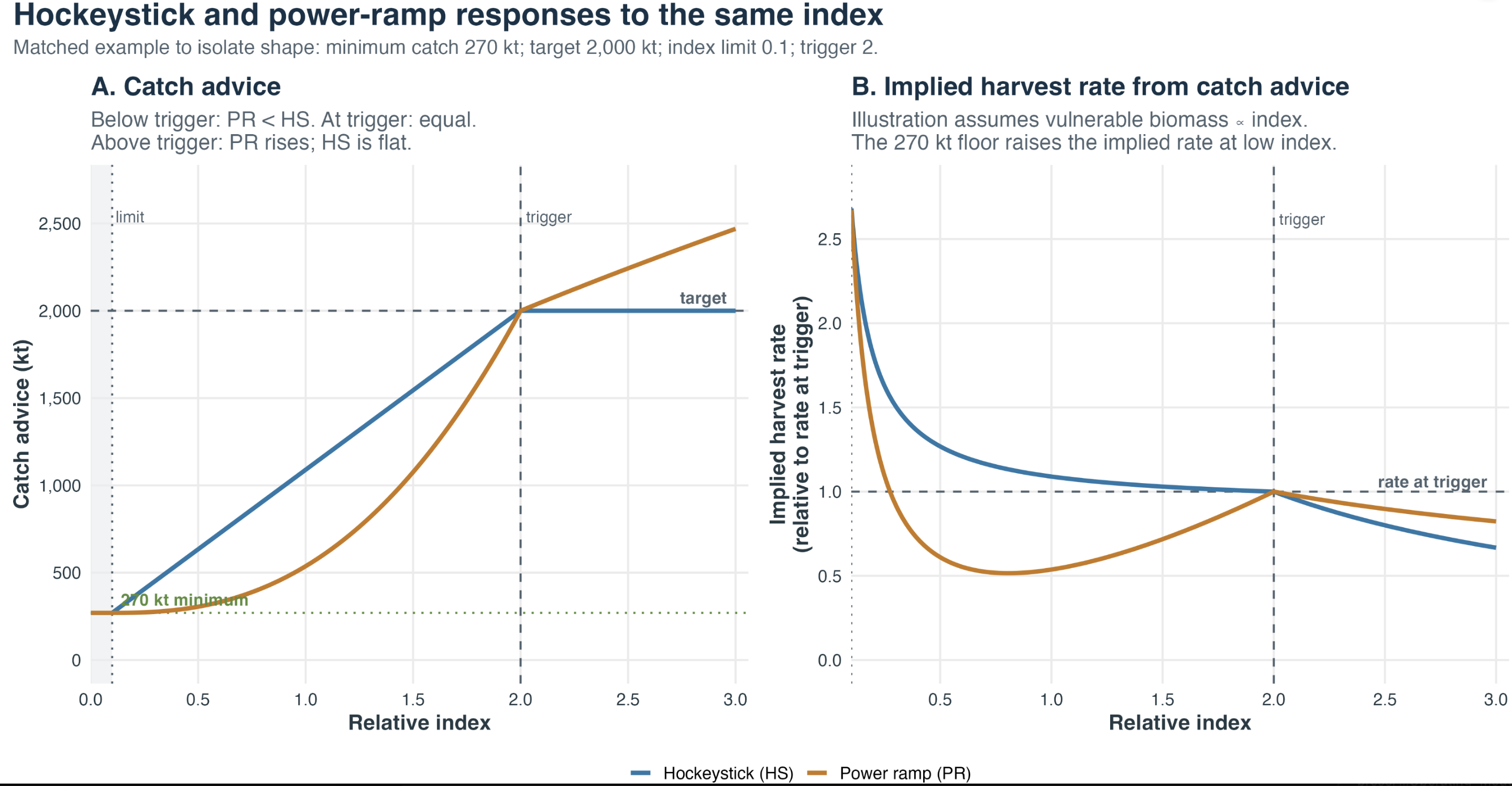
The matched example in Figure 3 isolates the effect of HCR shape by assigning both rules the same minimum, target, limit, and trigger. The hockey-stick increases catch advice linearly and then remains at its target. The power ramp is more conservative below the trigger but continues above the target when the index exceeds the trigger. Its second panel illustrates the harvest-rate pattern that would follow if vulnerable biomass were directly proportional to the index. For both HCR forms, the implied harvest rate rises at low stock sizes because catch advice is not allowed to fall below the 270-kt minimum; that fixed catch floor becomes an increasing proportion of the vulnerable biomass as stock size declines. The panel is explanatory rather than an estimated performance result or an additional rule used by the CMPs.
| Working label | Legacy ID | HCR family | Target or breakpoint (kt) | Tuned trigger | Annual decrease/increase limits |
|---|---|---|---|---|---|
| HS+20 | MP29 | Hockey-stick | 2,000 | 2.125 | -15% / +20% |
| HS-20 | MP43 | Hockey-stick | 2,000 | 1.9375 | -20% / +15% |
| HSsym | MP45 | Hockey-stick | 2,000 | 2.0625 | -15% / +15% |
| HS-30 | MP47 | Hockey-stick | 2,000 | 2 | -30% / +20% |
| PR+20 | MP32 | Power ramp | 1,500 | 1.640625 | -15% / +20% |
| PR-20 | MP44 | Power ramp | 1,500 | 1.6015625 | -20% / +15% |
| PRsym | MP46 | Power ramp | 1,500 | 1.625 | -15% / +15% |
| PR-30 | MP48 | Power ramp | 1,500 | 1.578125 | -30% / +20% |
The 500-draw refinement began from the earlier 100-draw tuned controls rather than restarting from a broad search. It then evaluated nearby trigger values under one saved OM and common random-number configuration. The resulting dynamic Kobe-green probabilities for HS+20, HS-20, HSsym, HS-30, PR+20, PR-20, PRsym, and PR-30 are 61.0%, 59.2%, 60.4%, 60.4%, 60.3%, 59.8%, 59.5%, and 60.6%, respectively.
A completed local trigger check tested one grid step below and above every selected control using the same saved 500 draws. The steps were 0.0625 for the hockey-stick rules and 0.03125 for the power-ramp rules, matching the final bisection resolution for each family. All eight checks behaved as expected: a higher trigger produced a higher long-term Kobe-green probability and a lower trigger produced a lower probability. Across the eight CMPs, one lower step changed the probability by -1.36 to -1.74 percentage points and one upper step changed it by +1.10 to +1.84 points. In plain language, this is a local tolerance profile: it checks how much the tuning result changes after a small move on either side of the chosen trigger, rather than assuming the selected number is uniquely precise. The full values are saved in the trigger-tolerance summary.
The hockey-stick increases advice linearly between the limit and trigger and then reaches a plateau. The power ramp reduces catch more quickly when the indicator is below its trigger and can continue to increase above its stated breakpoint according to the implemented rule. These structural differences, not the labels alone, create the main responsiveness-versus-stability contrast.
The completed 500-draw refinement is a higher-replication evaluation of the same conceptual CMPs, not a new set of procedures. Its controls and performance outputs are now the common basis for the candidate summaries in this report.
4.4 Annual TAC-change variants
The base CMPs limit annual advice to a 15% decrease and a 20% increase. The task team identified a limited set of alternatives for retuning and comparison, summarized in Table 6.
| HCR family | Base | Reverse asymmetry | Symmetric | Larger decrease |
|---|---|---|---|---|
| Hockey-stick | HS+20: -15%/+20% | HS-20: -20%/+15% | HSsym: -15%/+15% | HS-30: -30%/+20% |
| Power ramp | PR+20: -15%/+20% | PR-20: -20%/+15% | PRsym: -15%/+15% | PR-30: -30%/+20% |
The variants change both management responsiveness and the tuned trigger. They should therefore be compared as complete, retuned CMPs. The available 500-draw reference and nine-OM robustness runs support the common higher-replication comparison reported here.
The following reference-OM plot shows 15 reproducibly selected simulation iterations for the two hockey-stick asymmetry cases over 2025–2050. Iteration IDs are paired exactly across panels: for example, iteration 6 would be shown for both MPs if selected, and every selected ID occurs once in each panel. Each iteration has its own line color, and the same iteration uses the same color in both panels. HS-20 is MP43 (tun43), with annual limits of -20%/+15%; HS+20 is MP29 (tun29), with limits of -15%/+20%. The vertically stacked panels share a common catch scale, as shown in Figure 4.
4.5 Choice of indices
A CPUE/fishery-index-only comparison was more responsive but produced slightly lower short-term catch and higher short-term catch variability. The task team retained all five indices for the current focal comparison. The northern Chile acoustic survey is the only fishery-independent abundance index in the set and provides information that fishery-dependent series cannot fully replace. Conversely, equal weighting across regions can become problematic if northern and southern components diverge. These two findings support retaining the acoustic series while also monitoring regional index groups separately.
5 Performance evaluation and the draft scorecard
5.1 Performance framework
SCW17 agreed that CMPs should be evaluated across safety, yield, stability, and feasibility rather than by the tuning target alone. Tuning several CMPs to the same Kobe-green objective makes that objective a control for comparison, not a sufficient ranking statistic. The full performance framework can include:
- probabilities of dynamic Kobe-green, low biomass, overfishing, and stock collapse;
- spawning biomass, vulnerable biomass, and fishing pressure relative to reference points;
- short-, medium-, and long-term catch;
- interannual catch change and the frequency with which TAC-change limits bind;
- low-catch, minimum-catch, and fishery-shutdown-like outcomes;
- effort or catchability feasibility diagnostics; and
- robustness measures across individual OMs and stress tests.
A short headline table can aid Scientific Committee review, but the complete metric set and underlying distributions should remain available in the technical annex and interactive outputs.
The augmented candidate exports include vulnerable biomass relative to its 2025 level and relative to equilibrium vulnerable biomass at the fishing mortality that produces MSY. Vulnerable biomass was selected to provide a performance measure related to the fish available to the fishing fleet under the modeled selectivity, complementing spawning-biomass measures of biological stock condition. Reference-OM results are shown in Figure 5 and the corresponding robustness results in Figure 6.
5.2 Performance metrics by CMPs
The quilt in Figure 7 is an unweighted comparison of the eight annual-change variants listed in Table 5 under the reference OM. Annual values were averaged over 2041–2050 within each simulation iteration; cell labels are medians of those iteration means. Color is normalized independently within each metric across the eight variants.
Purple means lower relative preference and light lavender means higher relative preference (0 is darkest; 1 is lightest). Higher \(SB/SB_{\mathrm{MSY}}\), catch, \(VB/VB_{2025}\), and \(VB/VB_{\mathrm{MSY}}\) are treated as better; lower \(F/F_{\mathrm{MSY}}\), IACC, dynamic Kobe-red probability, probability of catch below 270 kt, and mean annual catch reduction are treated as better. Lower \(F/F_{\mathrm{MSY}}\) represents lower fishing pressure, while catch is shown separately. The within-column color scale is not an absolute biological or management threshold and must not be interpreted as a rank or recommendation.
The Kobe-red probability uses the same dynamic biomass denominator as the tuning objective: the equilibrium \(SB_{\mathrm{MSY}}/SB_0\) fraction is applied to projected unfished spawning biomass in each year and iteration. The low-catch probability is the proportion of all valid iteration-year catch outcomes below 270 kt during 2041–2050. Thus, if 10% of iterations are below 270 kt for five of the ten years and all are above it for the other five, the reported probability is 5%. Mean catch reduction averages positive annual percentage reductions during 2026–2050. Kobe-red probability and mean catch reduction are included in the illustrative composite score below. The low-catch diagnostic remains displayed but is not included in the worked composite until its management weight is reviewed. Kobe-green probability is omitted from the quilt because it is already the common tuning objective and provides little independent contrast among the closely tuned CMPs.
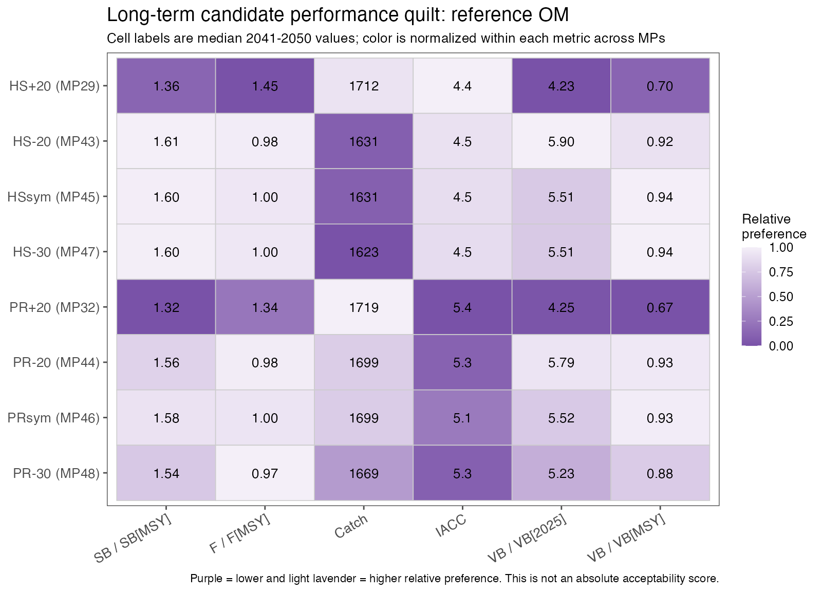
The underlying values, preferred directions, metric ranges, and normalized scores are saved in candidate_quilt_reference_summary.csv. An editable scorecard input layer is saved in candidate_scorecard_input_reference.csv. It converts quilt relative preference to a 0–100 benefit score, records the preferred direction and raw value, and supplies editable include and weight columns. The default weight is one for every metric, but no weighted total is calculated in this export. Changing weights or aggregating scores remains an explicit user decision under the method below.
5.3 Extensible weighted-scorecard method
The scorecard should be read as three connected layers, with no layer replacing the one before it:
- Raw performance and uncertainty. Report the performance statistic in its original units together with its simulated distribution or an appropriate interval. This is the primary results layer and includes, for example, catch in kt, biomass and fishing-pressure ratios, probabilities, and IACC. The boxplots and uncertainty bars elsewhere in this report provide examples. Point estimates alone are insufficient where CMP distributions overlap.
- Threshold- or target-based absolute performance. Where the Scientific Committee or Commission has agreed a biologically or operationally meaningful target and limiting boundary, performance can be expressed relative to those fixed reference values. Potential applications include dynamic Kobe probabilities, biomass thresholds, low-catch risk, and an agreed tolerance for interannual catch variability. The target, limiting boundary, direction, time window, and treatment of uncertainty must be specified before calculating this layer; they must not be inferred from the candidate results.
- Range-normalized relative preference. For metrics without agreed absolute targets, the quilt can scale each CMP between the least and most preferred observed values. This supports comparison across unlike units but describes position within the current candidate set, not absolute performance or acceptability.
For an absolute higher-is-better metric with agreed limiting boundary \(L_m\) and target \(T_m>L_m\), one possible transparent score is
\[ a_{jm}=\min\!\left(1,\max\!\left(0, \frac{x_{jm}-L_m}{T_m-L_m}\right)\right). \]
For a lower-is-better metric with \(T_m<L_m\), the numerator and denominator are reversed: \(a_{jm}=\min(1,\max(0,(L_m-x_{jm})/(L_m-T_m)))\). These forms are illustrative; an agreed probability, risk tolerance, or other metric-specific function may be preferable. Unlike min–max normalization, fixed \(L_m\) and \(T_m\) values permit comparison across candidate sets and report versions.
The current worked scorecard implements Layer 3, using the performance quilt in Figure 7 as a reproducible relative trade-off calculation for the eight candidate variants under the reference OM. It does not yet calculate Layer 2 absolute scores because the necessary metric-specific targets and limiting boundaries have not been agreed. Let \(x_{jm}\) be the value for CMP \(j\) and metric \(m\), and let \(x_m^{\min}\) and \(x_m^{\max}\) be the minimum and maximum across the included CMPs. The directionally normalized preference score \(p_{jm}\) is
\[ p_{jm} = \begin{cases} \dfrac{x_{jm}-x_m^{\min}}{x_m^{\max}-x_m^{\min}}, & \text{if higher values are preferred},\\[6pt] \dfrac{x_m^{\max}-x_{jm}}{x_m^{\max}-x_m^{\min}}, & \text{if lower values are preferred}. \end{cases} \]
Thus \(p_{jm}=0\) is the least preferred observed value and \(p_{jm}=1\) is the most preferred observed value for that metric and comparison set. It is a relative-preference score, not an acceptability score. If all CMPs have the same value for a metric, they are tied at \(p_{jm}=1\). With inclusion indicator \(I_m\) and non-negative weight \(w_m\), the aggregate score is
\[ S_j = 100\, \frac{\sum_m I_m w_m p_{jm}} {\sum_m I_m w_m}. \]
The companion Slick Spider (radar) view applies a higher-is-better orientation to its displayed metrics and repeats the 0–1 normalization within each selected OM. It is useful for seeing how the shape of CMP trade-offs changes among OMs, but radar shapes from different OMs do not show absolute changes in performance because each OM is scaled separately.
The contribution of metric \(m\) to the total is \(C_{jm}=100 I_m w_m p_{jm}/\sum_m I_m w_m\), so \(S_j=\sum_m C_{jm}\). The R implementation reads the editable Figure 7 input, checks that every CMP has one value for every included metric, and writes both the totals and metric-level contributions.
The worked results in Table 7 include eight metrics from Figure 7: the established six plus Kobe-red probability and mean catch reduction. The low-catch diagnostic remains a visible input with include = FALSE. The equal-weight view assigns one-eighth to every included metric. The balanced view assigns half the total weight equally across Catch, IACC, and mean catch reduction, and half equally across \(SB/SB_{\mathrm{MSY}}\), \(F/F_{\mathrm{MSY}}\), \(VB/VB_{2025}\), \(VB/VB_{\mathrm{MSY}}\), and Kobe-red probability. All inputs use the reference OM and the 2041–2050 summary window used in Figure 7, except mean catch reduction, which summarizes reductions over 2026–2050.
The spread among CMP point estimates is highly unequal among these metrics. Across the eight CMP medians, the coefficient of variation \(CV_m=sd_j(x_{jm})/|\bar{x}_m|\) is 51.2% for IACC, compared with 1.4% for Catch, 1.5–2.3% for the four biomass and fishing-pressure ratios, 6.9% for Kobe-red probability, and 38.3% for mean catch reduction. Within the hockey-stick and power-ramp families, IACC CVs are 7.9% and 3.9%, respectively. Consequently, ordinary min–max normalization visually expands small absolute contrasts in Catch and stock condition to the same 0–1 range as the much larger contrasts in IACC and mean catch reduction.
To expose this issue, Table 7 provides a reproducible dispersion-weighted sensitivity. For this calculation, the weight for metric \(m\) is
\[ w_m^{CV}=\frac{\sqrt{CV_m}}{\sum_k\sqrt{CV_k}}. \]
The square root moderates the dominance that would result from weighting directly in proportion to CV. With the current CMP set, the resulting weights are 31.4% for IACC, 27.1% for mean catch reduction, 11.5% for Kobe-red probability, 6.6% for \(VB/VB_{2025}\), 6.4% for \(VB/VB_{\mathrm{MSY}}\), 6.3% for \(F/F_{\mathrm{MSY}}\), 5.4% for \(SB/SB_{\mathrm{MSY}}\), and 5.3% for Catch. These weights answer which metrics most strongly distinguish the current CMPs; they do not answer which outcomes management should value most. They must be recalculated if the CMP set changes.
| CMP | Equal weight | Balanced | Dispersion weighted |
|---|---|---|---|
| HS+20 (MP29) | 70.74 (1) | 70.66 (1) | 80.25 (1) |
| HSsym (MP45) | 62.81 (2) | 65.51 (2) | 77.98 (2) |
| PR-20 (MP44) | 48.63 (3) | 46.37 (4) | 29.69 (5) |
| HS-30 (MP47) | 47.65 (4) | 52.34 (3) | 66.27 (3) |
| PRsym (MP46) | 43.27 (5) | 41.28 (5) | 29.42 (6) |
| HS-20 (MP43) | 32.73 (6) | 41.12 (6) | 60.08 (4) |
| PR-30 (MP48) | 25.14 (7) | 20.11 (8) | 18.03 (8) |
| PR+20 (MP32) | 23.25 (8) | 21.46 (7) | 18.27 (7) |
The machine-readable totals, including the dispersion-weighted sensitivity, are in candidate_scorecard_result_reference.csv, and the individual weighted contributions are in candidate_scorecard_contributions_reference.csv. These values are a reproducible calculation, but all three orders remain illustrative relative trade-offs rather than management rankings or acceptability scores: none of the weighting schemes is an agreed statement of management priorities, and the scores are relative to this candidate set.
The current worked scorecard based on Figure 7 is an illustrative framework, not the final scorecard. It contains eight CMPs and nine displayed performance metrics, eight of which are included in the worked composite scores. Please note:
- candidate rows can be added, removed, or replaced as the shortlist evolves;
- performance columns can be added as further safety, yield, stability, feasibility, and robustness metrics are validated;
- preferred direction, units, periods, transformation, and weight must be recorded for every metric; and
- normalization must be recalculated whenever the candidate set changes.
Min–max normalization is relative to the alternatives included. Adding or removing a CMP can therefore change every normalized score even when underlying MSE results do not change. This sensitivity is especially important here: because all eight CMPs have been tuned close to the same 60% dynamic Kobe-green objective, a narrow absolute range can still be stretched across the full 0–1 relative-preference scale. Absolute distances from agreed targets and the uncertainty in the raw outcomes are therefore more informative than min–max ordering when candidates are closely clustered. Weights express management priorities and should be agreed and recorded rather than presented as scientific constants. A weighted score is a decision aid, not a recommendation, and should always be shown with the Layer 1 underlying values and uncertainty, any defensible Layer 2 absolute scores, and sensitivity analyses.
6 Main performance and robustness findings
6.1 Biological requirements and the complete OM table
The approximately 60% dynamic Kobe-green probability used for tuning is a common comparison control, not a complete safety standard. The earlier COMM8 draft management objective included both a probability of being above \(B_{\mathrm{MSY}}\) in 2030 and a higher-probability requirement to remain above \(B_{\mathrm{lim}}\) during 2025–2040. The later K60 pathway supplied the common long-term Kobe-green tuning target. The present results should therefore be used to ask SC14 which biomass-limit, overfishing, time-specific, and component-specific requirements must be met; K60 should not be interpreted as having replaced every earlier objective unless SC14 records that decision.
The complete machine-readable table contains 112 CMP, OM, and stock-component rows and is available as candidate_biological_decision_table.csv. It was generated directly from the checked 500-draw Slick release with R/build_sc14_review_evidence.R. It reports long-term dynamic Kobe-green probability, three ways of describing the chance that spawning biomass falls below dynamic \(SB_{\mathrm{MSY}}\), overfishing probability, catch, and IACC. These are candidate diagnostics for discussion, not agreed limit-reference criteria. All eight CMPs remain not ready for annual use because their final operational specifications are incomplete.
| OM | Stock | CMP | P(green) | P(any SB < 1) | P(F > 1) | Catch | IACC |
|---|---|---|---|---|---|---|---|
| om11 | CJM | HS+20 | 61.0% | 45.2% | 37.0% | 1570.8 | 5.5 |
| om11 | CJM | HS-20 | 59.2% | 47.2% | 38.7% | 1552.0 | 5.6 |
| om11 | CJM | HSsym | 60.4% | 45.4% | 37.4% | 1557.9 | 5.4 |
| om11 | CJM | HS-30 | 60.4% | 46.4% | 37.5% | 1568.7 | 6.0 |
| om11 | CJM | PR+20 | 60.3% | 52.0% | 36.6% | 1881.5 | 10.5 |
| om11 | CJM | PR-20 | 59.8% | 52.2% | 36.4% | 1923.2 | 10.7 |
| om11 | CJM | PRsym | 59.5% | 52.0% | 37.5% | 1914.4 | 10.1 |
| om11 | CJM | PR-30 | 60.6% | 53.2% | 33.8% | 1865.6 | 11.6 |
| om23 | North | HS+20 | 1.1% | 99.0% | 98.9% | 4.2 | 0.6 |
| om23 | North | HS-20 | 0.9% | 99.0% | 99.1% | 3.2 | 0.3 |
| om23 | North | HSsym | 1.0% | 99.0% | 99.0% | 3.8 | 0.5 |
| om23 | North | HS-30 | 1.0% | 99.0% | 99.0% | 3.5 | 0.4 |
| om23 | North | PR+20 | 2.7% | 97.4% | 97.2% | 10.3 | 1.6 |
| om23 | North | PR-20 | 2.9% | 97.0% | 97.1% | 11.2 | 1.8 |
| om23 | North | PRsym | 2.7% | 97.2% | 97.2% | 10.8 | 1.7 |
| om23 | North | PR-30 | 2.7% | 97.2% | 97.3% | 10.1 | 1.6 |
| om23 | Southern | HS+20 | 100.0% | 0.0% | 0.0% | 1284.5 | 4.5 |
| om23 | Southern | HS-20 | 99.9% | 0.0% | 0.1% | 1304.2 | 4.3 |
| om23 | Southern | HSsym | 100.0% | 0.0% | 0.0% | 1291.0 | 4.4 |
| om23 | Southern | HS-30 | 99.9% | 0.0% | 0.1% | 1297.9 | 4.4 |
| om23 | Southern | PR+20 | 100.0% | 0.0% | 0.0% | 1234.0 | 6.6 |
| om23 | Southern | PR-20 | 100.0% | 0.0% | 0.0% | 1243.4 | 6.4 |
| om23 | Southern | PRsym | 100.0% | 0.0% | 0.0% | 1237.0 | 6.2 |
| om23 | Southern | PR-30 | 100.0% | 0.0% | 0.0% | 1250.1 | 6.8 |
The om23 result requires particular attention. For its northern component, long-term dynamic Kobe-green probability is only 0.9–2.9% across the eight CMPs in the current checked release, while the probability of falling below dynamic \(SB_{\mathrm{MSY}}\) in at least one year is 97.0–99.0%. This is a model/configuration sensitivity rather than a forecast, but it must not be hidden by pooling OMs or stock components. SC14 should explicitly record whether om23 is decisive, a concern requiring additional protection or analysis, or too implausible to determine selection.
6.2 Reference comparison
The illustrative reference-OM scorecard in Table 7 provides the current eight-CMP comparison. HS+20 ranks first and HSsym second under all three schemes. Adding Kobe-red probability and mean catch reduction moves HS-30 to third under the balanced and dispersion-weighted schemes. The dispersion-weighted result then places HS-20 fourth, followed by PR-20, PRsym, PR+20, and PR-30. The equal-weight and balanced columns show how several of these middle positions change when metric emphasis changes. The separation between the two +20 sensitivity CMPs shows why an analytical role should not be confused with a shared performance ranking.
This ordering is illustrative and relative to the CMPs, metrics, directions, 2041–2050 window, and weights included in the scorecard. It does not mean that one CMP dominates every biological, yield, stability, and responsiveness objective. The underlying values and trade-off figures should therefore remain the basis for interpreting why the order changes with management priorities.
6.3 Reference set trade-offs
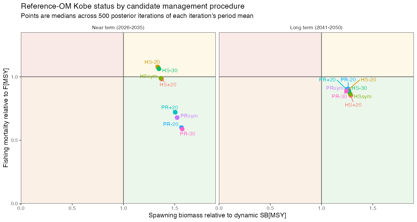
Kobe status. Figure 8 provides the direct reference-OM comparison of spawning-biomass status and fishing pressure for the near-term (2026–2035) and long-term (2041–2050) periods. Within each posterior iteration, each ratio is averaged over the stated period; points are the medians of those period means across the 500 iterations. The vertical and horizontal lines at 1 define the conventional Kobe quadrants.
Spawning biomass. The reference-set yield–spawning-biomass comparison uses mean catch during 2026–2030 and mean \(SB/SB_{\mathrm{MSY}}\) during 2036–2040. Points show means among 500 draws, and horizontal and vertical bars show the separate 10th–90th percentile ranges for the two measures.
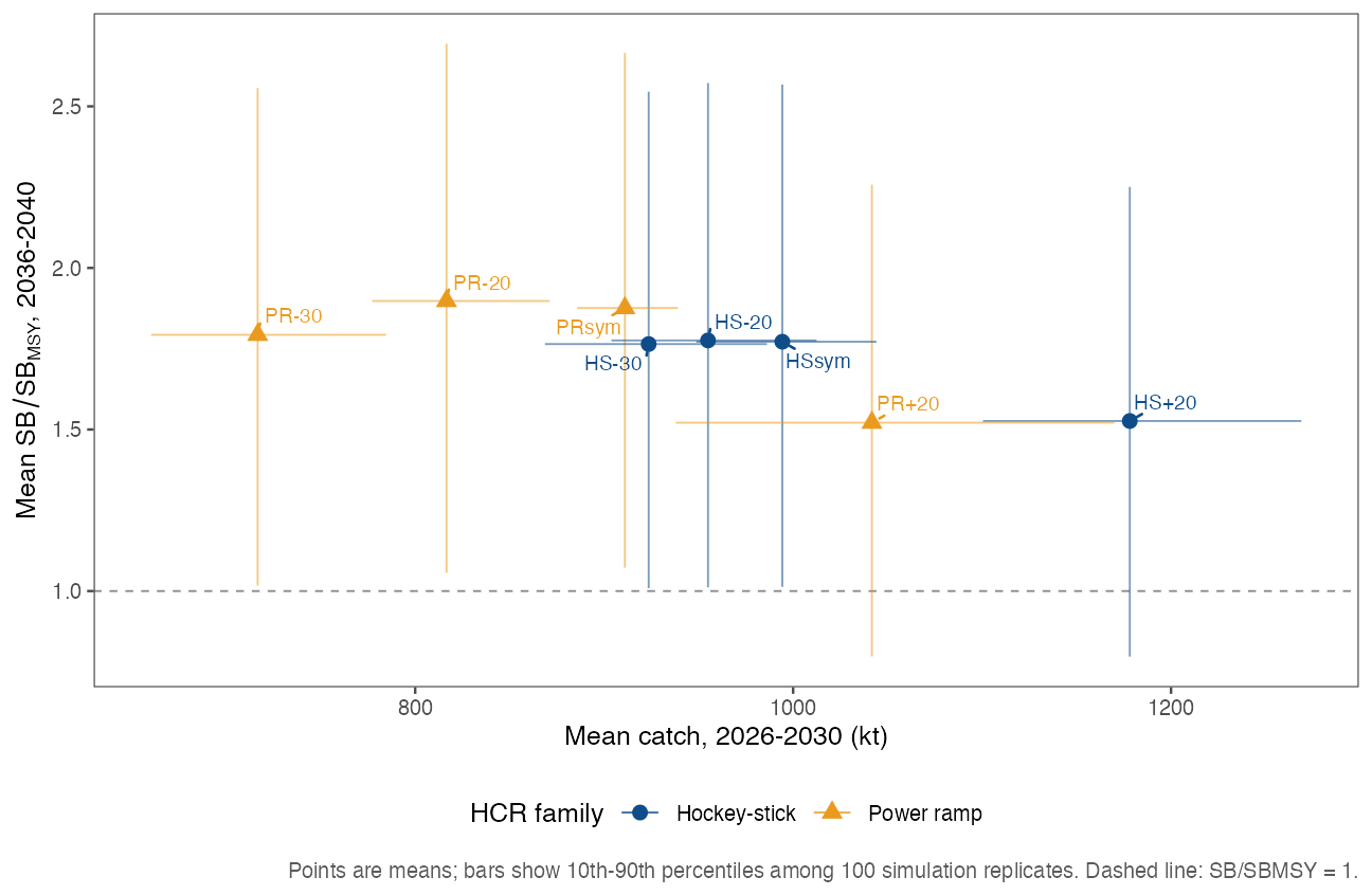
Figure 9 shows the reference-OM pattern. The hockey-stick CMPs generally occupy the higher-catch, lower-biomass part of the plot, while the power-ramp CMPs generally produce lower catch and higher biomass. Responses to the annual-change variants are not monotonic across the two families because each variant includes a separately tuned trigger as well as different change limits. The uncertainty ranges overlap substantially, so the plot should not be read as a deterministic ranking.
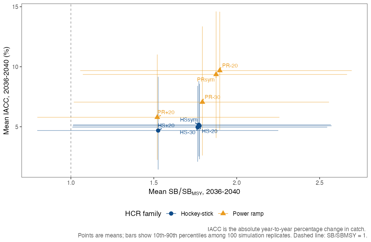
Figure 10 provides a complementary reference-OM view of biological status and catch stability. The horizontal axis is the replicate mean \(SB/SB_{\mathrm{MSY}}\) during 2036–2040. The vertical axis is mean IACC during the same period, where annual IACC is \(100|C_t/C_{t-1}-1|\): the plotted period therefore covers the five annual changes from 2035–2036 through 2039–2040. Lower IACC indicates more stable catch. Points are means among 500 draws; horizontal and vertical bars are the separate 10th–90th percentile ranges of the replicate-level period means. As in Figure 9, overlap is substantial and the marginal bars do not show within-replicate covariance.
The marked difference in IACC between the four hockey-stick and four power-ramp CMPs is not caused by different calculations. For every CMP and year, IACC is calculated identically as \(100|C_t/C_{t-1}-1|\); an independent recalculation from the saved annual catch series reproduced every stored IACC value exactly. The pattern reflects HCR structure. Hockey-stick advice reaches a constant 2,000-kt target above its trigger, producing many years with essentially no catch change. The power ramp has no equivalent upper plateau: advice continues to respond to changes in the combined indicator above its trigger, so catch can vary even when the stock is on the upper branch of the rule. Over 2041–2050, mean IACC is about 5.4–6.0% for the hockey-stick CMPs and 10.1–11.6% for the power-ramp CMPs. The quilt values are somewhat different because Figure 7 reports the median across iteration-specific period means rather than the mean across all iteration-years. This structural family contrast is a genuine stability trade-off, but it also means that a highly weighted IACC column can strongly influence a composite score; the raw IACC distributions and HCR shapes should therefore remain visible alongside any weighted summary.
6.4 Trade-offs under robustness cases
6.4.1 Recruitment stress
The discrete recruitment crash and seven-year cyclic reduction lowered long-term catch and increased catch variability for both central CMPs. PR+20 responded more quickly and produced comparatively stronger long-term recovery in these tests, while HS+20 retained the relative stability advantages seen in the reference case. These are robustness contrasts, not forecasts that either recruitment path will occur.
6.4.2 Alternative selectivity
The alternative-selectivity OM exposed younger and smaller fish to greater fishing pressure. Similar catch levels could then occur with lower spawning biomass and poorer Kobe performance. In the completed results, HS+20 retained higher catch while PR+20 retained higher spawning biomass; this is a trade-off, does not show that either CMP is uniformly better. Interpretation is also affected by the changed \(F_{\mathrm{MSY}}\) reference point.
6.4.3 Two-stock hypotheses and catch distribution
In the two-stock OM without movement, the southern component remained above the agreed benchmark while the northern component did not. An exploratory shift of ~3% in simulated catch distribution from north to south brought both components to the 60% long-term benchmark. This illustrates sensitivity to spatial exploitation; it is not an allocation or catch-distribution recommendation.
In the movement OM, biomass transferred from the southern to the northern component. Because the five indices were combined with equal weights, increasing northern indices could raise the overall indicator while southern spawning biomass declined. No tested time-invariant catch distribution resolved the long-term benchmark for both components. The test is deliberately stressful and does not establish that this movement process is occurring. It does establish a management-relevant warning signal: persistent divergence between northern and southern indices.
Spawning biomass. The saved results also support yield–spawning-biomass comparisons across the single-stock and two-stock robustness cases.
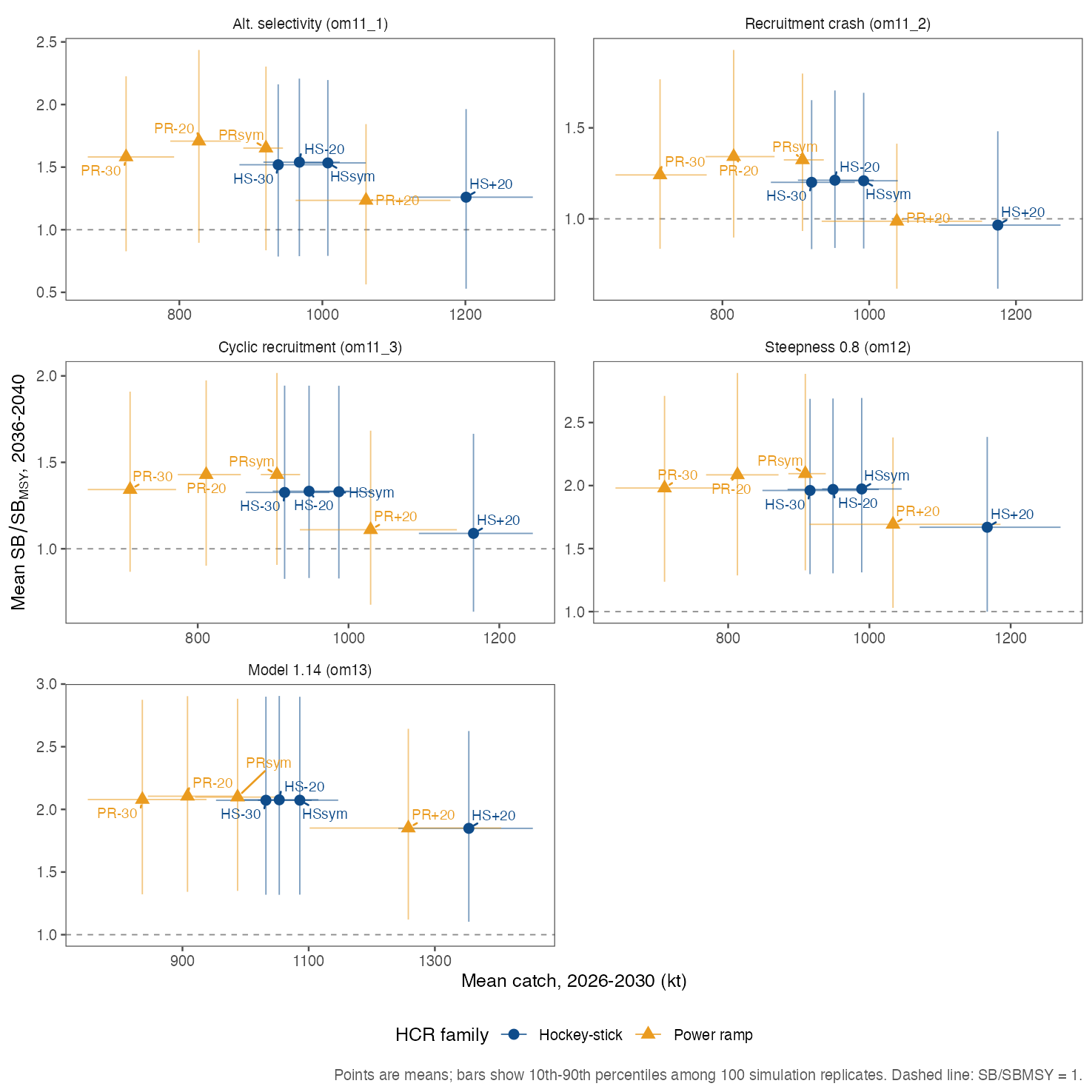
The same broad direction is visible across the single-stock robustness cases (Figure 11), but the location and separation of configurations changes by OM. Recruitment stress reduces later biomass and changes the apparent trade-off, while productivity and assessment-configuration alternatives move both axes.
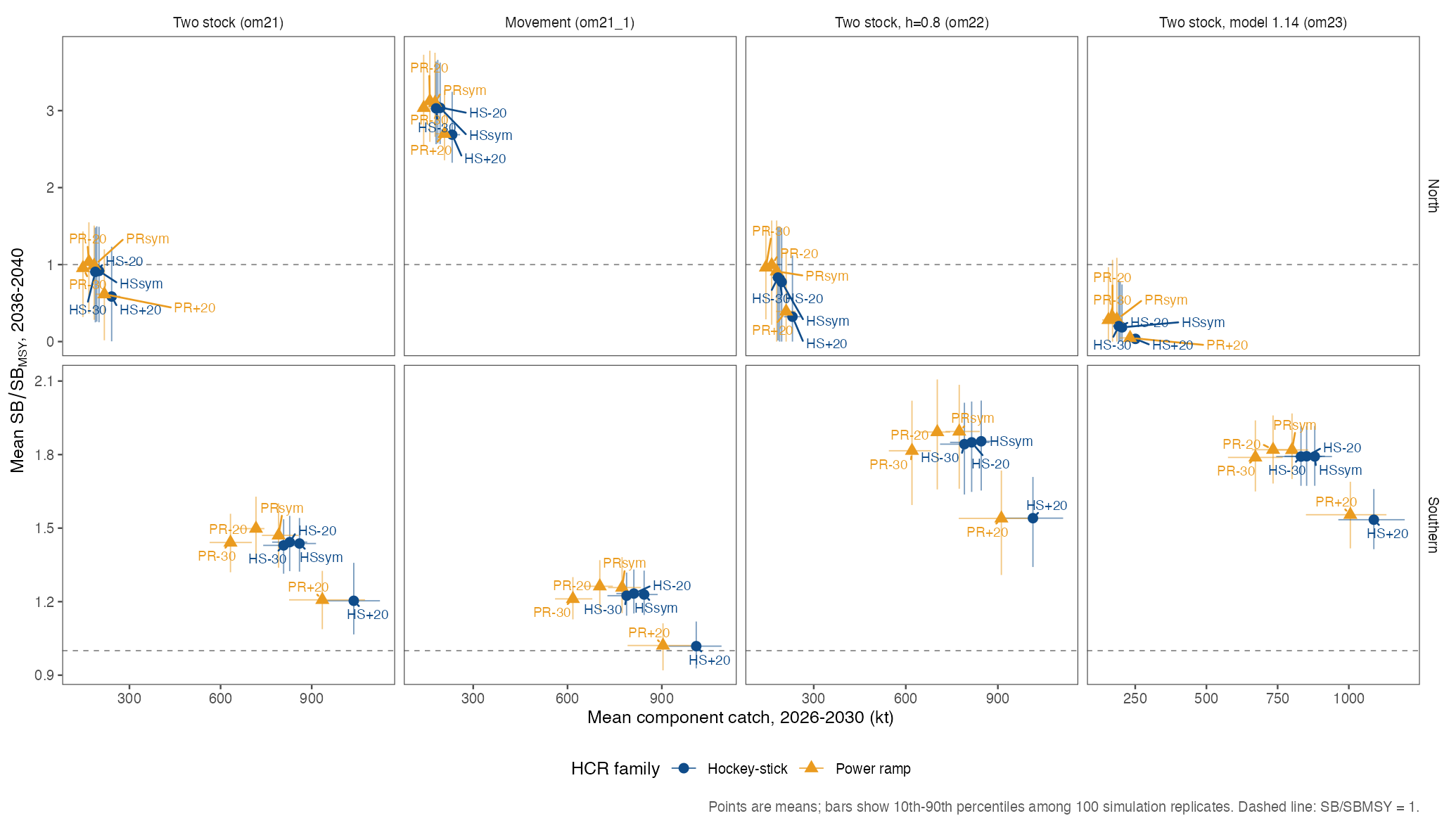
For the two-stock cases (Figure 12), each row is a biological component and the horizontal axis is component catch, not total catch. The plots therefore diagnose stock-specific consequences and must not be interpreted as an allocation comparison. They reinforce the need to keep northern and southern outcomes separate.
The spawning-biomass figures in Sections 6.2 and 6.3 use the completed 500-draw comparison but remain selective summaries for three reasons. First, the x and y uncertainty bars are marginal percentiles and do not show the within-replicate covariance between plotted measures. Second, spawning biomass is shown relative to each draw’s equilibrium SBMSY rather than in tonnes. This differs from the time-varying dynamic SBMSY denominator used for tuning and in Figure 8. Third, these views cover only selected yield, biological, and catch-stability periods; they do not include fishing pressure, Kobe-green probability, low-catch risk, feasibility, or the other performance measures needed for a decision. The plotted summary values are saved in doc/data/sc14-preliminary-tradeoffs.csv and can be regenerated with R/plot_sc14_tradeoffs.R.
7 Banking, borrowing, and implementation constraints
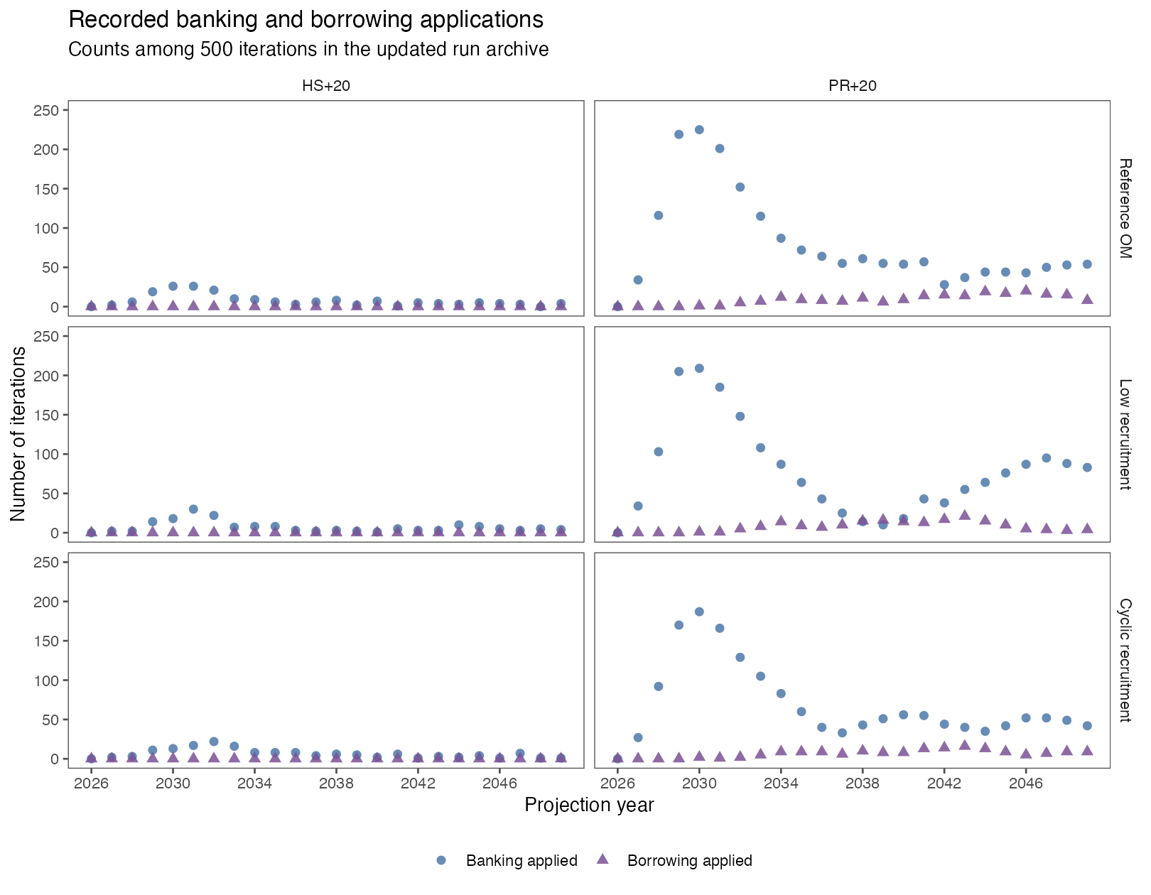
SCW17 treated banking and borrowing as a sensitivity to apply to the final CMP set rather than as feedback within the HCR. Updated 500-iteration results are now available for HS+20 and PR+20 under the reference, low-recruitment, and cyclic-recruitment OMs. The tested implementation used a 10% banking or borrowing amount when HCR advice changed by at least 15%, subject to the CMP-specific healthy-rule condition. In operational terms, a decline of more than 15% made an iteration eligible to borrow 10% of the new advice (adding it to the current TAC and deducting it subsequently), while an increase of more than 15% made it eligible to bank 10% (deducting it from the current TAC and making it available subsequently).
The current msemodules::bank_borrow.is() implementation also evaluates the recorded HCR branch against the CMP-specific healthy threshold. For HS+20 this requires rule status 3: the indicator is at or above the hockey-stick trigger and advice is on the constant target branch. For PR+20 it requires rule status 2: the indicator is at or above the power-ramp trigger and advice is on its upper branch. All recorded applications in the updated archive satisfy the applicable healthy-branch condition. These B&B runs did not retain the annual TAC-change limits, so comparison with the standard runs combines the effect of banking and borrowing with the effect of removing those limits.
The long-term results are summarized in Table 9. The values with B&B come from the supplied 500-iteration performance_babs.rds, whose six run identifiers match the updated babs.rds archive. Under the reference OM, mean SB0green during 2041–2050 was 0.582 for HS+20 and 0.464 for PR+20. The values under low recruitment were 0.416 and 0.489, respectively, and under cyclic recruitment were 0.409 and 0.455. The without-B&B values added in Iago Mosqueira’s contribution cover the same three OMs, but the comparison is not a controlled estimate of the incremental B&B effect because the B&B runs removed the annual TAC-change limits.
| OM | CMP | Without B&B | With B&B |
|---|---|---|---|
| Reference OM | HS+20 | 0.603 | 0.582 |
| Reference OM | PR+20 | 0.607 | 0.464 |
| Low recruitment | HS+20 | 0.508 | 0.416 |
| Low recruitment | PR+20 | 0.613 | 0.489 |
| Cyclic recruitment | HS+20 | 0.407 | 0.409 |
| Cyclic recruitment | PR+20 | 0.527 | 0.455 |
The spawning-biomass distributions for the six banking-and-borrowing runs in Table 9 are shown in Figure 13. Each boxplot summarizes the distribution across the 500 iterations after first averaging SB/SBMSY within each iteration over the stated period. This is a stock-status ratio, whereas SB0green in Table 9 is the probability of being in the dynamic Kobe green quadrant; the two summaries are complementary and should not be read as the same performance measure. The dashed line marks SB/SBMSY = 1.
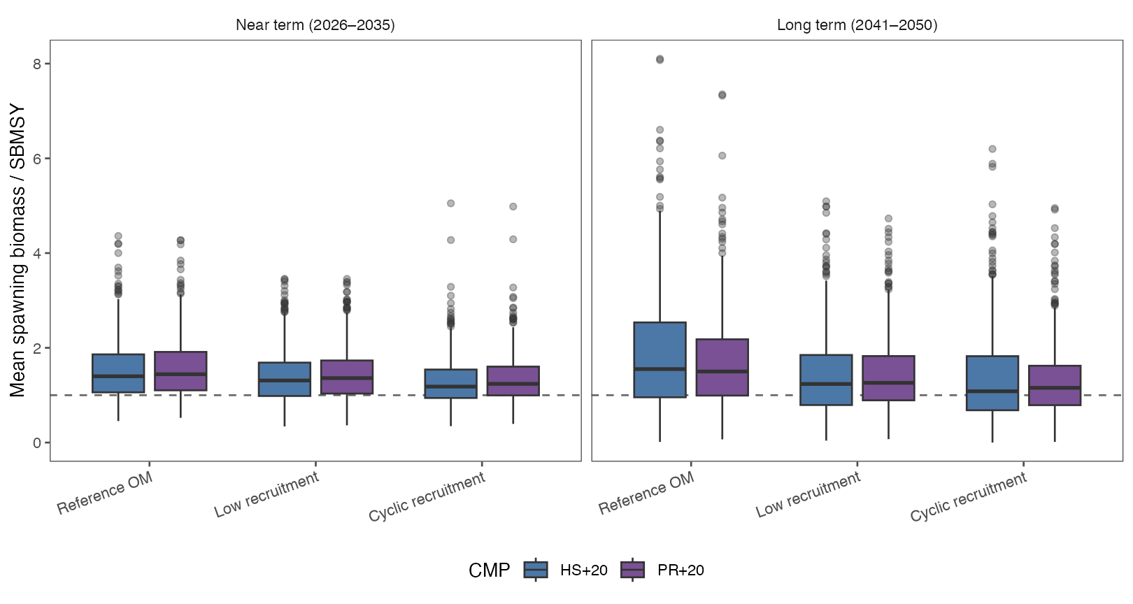
The updated archive resolves the earlier provenance problem: its six run names match the performance table, and its banking.isys and borrowing.isys tracking fields contain non-zero recorded applications. Figure 14 therefore counts transactions recorded in the run archive directly, rather than reconstructing eligibility from annual changes in HCR advice. The updated 500-iteration pattern is consistent in kind with the contractor’s earlier 100-iteration plot, while the exact counts differ because the simulation sample is larger and not the same set of draws.
If the intent is to estimate the incremental effect of banking and borrowing, the analysis still requires a matched no-B&B comparison using the same 500 OM draws and the same TAC-change-limit treatment.
Effort feasibility is another implementation constraint. A TAC can be mathematically available but difficult to catch when fish distribution or catchability changes. The OM includes an effort cap across all fisheries, set at three times the effort level of 2025, to prevent unrealistic projected effort. Low realized catch, catch-rate proxies, and the frequency of binding effort constraints should be retained as supporting diagnostics.
8 Exceptional circumstances and annual monitoring
An exceptional-circumstances protocol should identify when new information is inconsistent with the conditions under which a selected CMP performed acceptably. SCW17 considered the ECP software framework as a proof of concept: robustness simulations can identify data patterns associated with poor CMP performance, and detection rules can then be evaluated for false-positive and false-negative errors.
The current analysis identifies at least two monitoring priorities:
- persistent divergence between northern and southern abundance indicators, particularly in relation to the two-stock-with-movement hypothesis; and
- whether current survey, catch, and fishery information lies outside OM distributions or is associated with simulated CMP failure states.
Preliminary oral fishery updates reported at the 24 July meeting are not validated data submissions and do not by themselves establish exceptional circumstances. A protocol should specify the observations, data timing, triggering information, review authority, possible responses, and return-to-rule conditions before operational use.
9 Summary and conclusions
This MSE combines the operating-model development and management-procedure design undertaken before and during SCW17 with the subsequent implementation, tuning, robustness testing, and performance evaluation. The candidate procedures apply transparent hockey-stick and power-ramp HCRs to a combined indicator constructed from five standardized abundance series. A distinctive feature is that the OMs simulate uncertainty, temporal autocorrelation, and cross-correlation among those series, rather than treating multiple indicators as independent confirmations of stock change.
The analysis narrows the broader workshop set to two central rule families and reasonable annual TAC-change variants. Candidate performance is evaluated against a reference OM and a structured robustness set spanning productivity, recruitment stress, selectivity, stock structure, movement, and spatial catch distribution. The results demonstrate trade-offs among biological condition, catch, stability, and responsiveness rather than identifying a single CMP that dominates every objective. The performance quilt and worked scorecards provide transparent summaries, but the underlying distributions, metric definitions, weights, and robustness results remain necessary for interpretation. For example, MP29 and MP45 (HS+20 and HSsym) receive the two highest illustrative composite scores under the reference OM. That result is not a claim that either dominates across the robustness set: their relative performance still depends on the metric, weighting, and robustness scenario considered.
The external experts invited to SCW17 supported progressing the MSE. Tom Carruthers considered the framework suitable for testing CMPs, with a defensible reference OM, a comprehensive robustness set, relevant performance measures, and empirical CMPs comparable with procedures used in other fisheries. He concluded that the work was sufficiently advanced to support shortlisting defensible CMPs for Scientific Committee consideration and that the improvements still identified were not substantial enough to delay adoption of a robust management procedure. He also emphasized that MSE is an ongoing, iterative process in which the framework can be refined after an MP is adopted and applied.
David Miller and Rosana Ourens likewise viewed the benchmark assessment as a strong basis for the reference OM, the robustness set as covering important uncertainties, and the use of dynamic reference points and simple empirical index-based rules as sensible.
External-review caveats. Their comments also stated that CMP design would have benefited from more stakeholder input and that earlier agreement on the assessment and reference points would have kept the discussion more focused. Those caveats are retained here as reviewer findings.
Author response. Commission participants and other stakeholders received presentations and opportunities to provide input before and during the MSE process, including on management preferences and annual TAC-change limits. This history does not remove the reviewers’ caveats. It supports continued and better-documented stakeholder involvement, especially when narrowing the CMP set and setting weights or other management preferences.
The technically relevant priorities identified by the experts include accurately representing historical cross-correlation among indices, exploring alternative index combinations, and establishing a formal exceptional-circumstances framework. Taken together, the external review supports applying the MSE as a living management process, with monitoring, stakeholder input, and agreed revisions continuing after initial adoption rather than treating the current analysis as a one-time exercise.
The available work supports asking SC14 to identify a provisional shortlist for final comparative evaluation, accompanied by annual monitoring and a formal exceptional-circumstances process. It does not request Commission selection or adoption at this stage. Because this synthesis contains result-dependent statements, scores, and conclusions, the interactive scorecard explorer lets users compare CMPs, select performance metrics, apply alternative weighting schemes, and specify weights directly. The application complements rather than replaces the underlying performance distributions and documented management judgments.
The Scientific Committee is asked to consider the following:
Noting
- that the approaches provide valid combinations of the available information for application in the tested HCRs;
- that the work identifies reasonable annual TAC-change variants informed by polling of Commission members;
- that the current comparison addresses the K60 tuning pathway but SC14 still needs to state how the earlier COMM8 objectives and component-level risks should be applied;
- the use of all five indices and the complementary value of the fishery-independent acoustic series;
- that northern and southern indicators should continue to be tracked separately, as in the past, alongside the combined CMP indicator and monitored through the annual assessment process, including when evaluating whether exceptional circumstances may be occurring;
- that the updated 500-iteration banking-and-borrowing runs retain explicit transaction tracking and indicate a potentially material effect on MP performance, but require a matched no-B&B comparison before the incremental effect is interpreted for implementation; and
- that the robustness tests provide plausible scenarios for testing the CMPs.
Advising
- the analytical work as satisfying the request from the Commission;
- identification of a provisional shortlist for final comparative evaluation, without implying selection or adoption;
- development of a formal exceptional-circumstances protocol, including evaluation of detection performance and pre-agreed responses; and
- review and documentation of the full performance-metric set and any weighting process, while retaining the underlying outcomes rather than relying on a composite score alone.
10 Source, terminology, and interpretation notes
This synthesis uses “CMP” for a procedure still under evaluation and “MP” when referring to the identifiers used in the analysis. “Catch distribution” is used for two-stock sensitivity tests; those tests are not allocation advice. “Dynamic Kobe green” refers to performance calculated using the dynamic reference-point implementation described above.
Numerical values from presentations and meeting materials should be checked against the named final simulation archive before submission. Where a presentation takeaway and the later meeting interpretation differed in tone, this report follows the meeting’s more cautious interpretation. The meeting report itself was prepared from meeting notes, transcript material, and an automated meeting summary; preliminary oral information requires confirmation against formal submissions.
11 Sources
Mosqueira, Iago, and B. Bergès. 2026. Management Strategy Evaluation (MSE) for SPRFMO Jack Mackerel: Progress Since SCW17. Presentation. https://sprfmo.github.io/jmMSE26/evidence/presentation_20260725.pdf.
Punt, André E., Doug S. Butterworth, Carryn L. de Moor, José A. A. De Oliveira, and Malcolm Haddon. 2016. “Management Strategy Evaluation: Best Practices.” Fish and Fisheries 17 (2): 303–34. https://doi.org/10.1111/faf.12104.
SPRFMO. 2026. “Jack Mackerel MSE 2026 Project Site.” https://sprfmo.github.io/jmMSE26/.
SPRFMO Jack Mackerel MSE Task Team. 2026. Meeting Report: Candidate Management Procedures, Robustness Testing, and SC14 Preparation. South Pacific Regional Fisheries Management Organisation. https://sprfmo.github.io/jmMSE26/outputs/meeting-report-20260724/SC14_JM_MSE_meeting_report_2026-07-24.pdf.
SPRFMO Jack Mackerel Working Group. 2025. SC13-JM09 Report of the Management Strategy Evaluation (MSE) Workshop (SCW15). South Pacific Regional Fisheries Management Organisation. https://sprfmo.github.io/SCW15_report/.
SPRFMO Jack Mackerel Working Group. 2026a. JMWG Benchmark Meeting Report 2026. South Pacific Regional Fisheries Management Organisation. https://sprfmo.github.io/JM_SCW_prep/JMWG-Benchmark-Meeting-report-2026.html.
SPRFMO Jack Mackerel Working Group. 2026b. Report of the Jack Mackerel Management Strategy Evaluation Workshop—SCW17. South Pacific Regional Fisheries Management Organisation. https://sprfmo.github.io/scw17/SCW17-MSE-Workshop-report.html.
SPRFMO Jack Mackerel Working Group. 2026c. SCW17/Paper-01: Model Developments. South Pacific Regional Fisheries Management Organisation. https://sprfmo.github.io/scw17/SCW17-Paper-01-ModelDevelopments.html.